(Upload on October 18 2021) [ 日本語 | English ]
Mount Usu / Sarobetsu post-mined peatland
From left: Crater basin in 1986 and 2006. Cottongrass / Daylily
HOME > Lecture catalog / Research summary > Glossary > Diversity
[diversity index, species-area curve, biodiversity (生物多様性)]
|
Diversity: is evaluated by: evenness, heterogeneity (homogeneity), richness, stability or complexity Species richnessNumber of species in a given area, such as community and plotRelative abundance of species richness
Tropical → large number many → high species richness Diversity (Shmida & Wilson 1985)How the number of species is determined in a given commmunity or plot
Richness Functional diversitythe elements of biodiversity that influence how ecosystems functionPersistence (永続性)species composition does not change through time in the absence of stress and disturbanceResistance (耐性)no change with "shoves" - stress/disturbanceCommunity Resistance, R (Frank & McNaughton 1991) Rj = 1 - Σi=1m(Δpij/2)
pij: relative dominance of species ith in community j Resilience (復元性, 弾力性)the capacity of an ecosystem to recover from stress and disturbance = stability (s.s.)
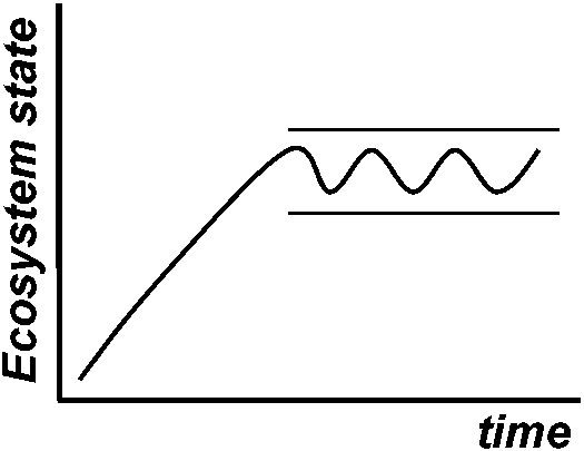
Stability within bounds = no recognizable major changes in vegetation community over time
loss of biodiversity may alter the ecosystem resilience |
Ex. effects of tephra on wetland vegetation (Hotes et al. 2010) Variability (変動性) ⇔ stability (安定性)fluctuating scale expressed by the deviation of density, etc. → small = stableHypotheses on the changes of species diversityS = f(+ habitat diversity, -(+) disturbance, + area, + age,+ matrix heterogeneity, - isolation, - boundary discreteness) S = number of species Manage for persistence Manage for changeEcosystems are still recognizable Ecosystems have fundamentally as being the same system (character) change to something differnt ⇐===================================================⇒ Resistance Resilience Transition  Fig. 1. Conceptual diagram of resistance, resilience and transition (Swanston et al. 2016; Nagel et al. 2017; Millar et al. 2007) Lottery model (富くじモデル)– no competitionIntermediate disturbance hypothesis, IDH (中規模撹乱仮説)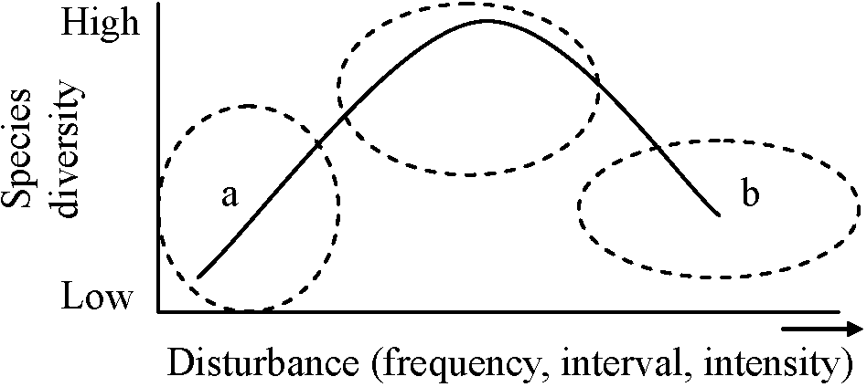
|
Diversity-stability hypothesis Hypothesis for the functional role of species diversity in ecosystem (Johnson, et al. 1996). Diversity-stability hypothesis: ecological communities increase in energetic efficiency (productivity), and in ability to recover from disturbance, as the number of species in the system increases (MacArthur 1955, Elton 1958). In its original form (MacArthur 1995), this hypothesis did not include assertions of linearity in the effect of species richness on ecosystem function. The following hypotheses are alternatives to this hypothesis (Kareiva 1994, Tilman & Downing 1994, Collins 1995, Baskin 1995, Walker 1995). |
Rivet hypothesis: likening species in an ecosystem to rivets holding an airplane together the removal of rivets beyond some threshold number may cause the airplane, or the ecosystem, to suddenly and catastrophically collapse (Ehrlich & Ehrlich 1981). Explicit in their presentation is the appreciation that a few extinctions may go unnoticed in terms of system performance because some species are redundant, generating a nonlinear relationship between species richness and ecosystem function. Redundancy hypothesis: certain species have some ability to expand their 'jobs' in ecosystems to compensate for neighbor species that go extinct, sensu Ehrlich & Ehrlich (1981), (Walker 1992). Species may be segregated into functional groups; those species within the same functional group are predicted to be more expendable in terms of ecosystem function relative to one another than species without functional analogs. Idiosyncratic hypothesis: the possibility of a null or indeterminate relationship between species composition and ecosystem function (Lawton 1994). This relationship is expected, for example, in communities featuring higher-order interactions. |
| Ecosystem | Disturbance type | Diversity measure | Productivity measure | Stability measure | Diversity/ productivity relationship | Diversity/ stability relationship |
| California annual grassland1 | Annual variation | Sa | SCa (aboveground) | SC(NPP)-1plants (-) | plants (0) | |
| New York old fields1 | Annual variation; N-P-K fertilizer | S/log2 N;S and H' | NPPa (aboveground, belowground) | ΔNPP | plants (-) herbivores (-) carnivores (-) (0) | plants (+) herbivores (-) carnivores (-) |
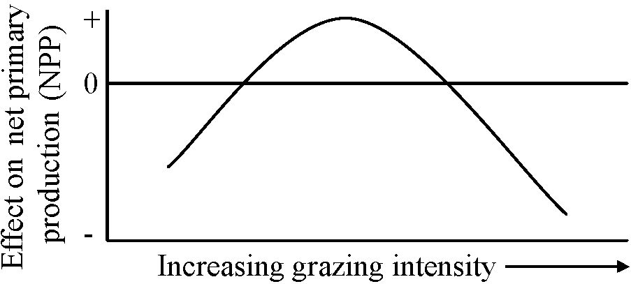
| Serengeti2 | Δprecipitation; grazing | H' | NPP (aboveground) | ΔSC | NAa | plants (+) |
| Yellowstone grasslands3 | drought; grazing | H' | SC (aboveground) | Δrelative abundances | NA | plants (+) |
| British grasslands4, 5 | fertilization; mowing; Δprecipitation | S | SC (aboveground) | Δvegetation; composition4 ΔSC4, 5 | plants (-) | plants (-)4, (-)4, 5 |
| Minnesota grasslands6, 7 | drought6, ΔS7 | S | SC (aboveground) | DSC; recovery rateb, NA7 | plants (-)6, (+)7 | plants (+)6, NA7 |
| Costa Rican tropical forest8 | annual variation | S | soil fertilityc | Δsoil fertility | NA | plants (+) |
| Ecotron9 | S | S | NPP | NA | plants (+) | NA |
|
a. S, species richness; SC, standing crop; NPP, net primary production; N, total community biomass; Δ, change in parameter, H', Shannon index; NA, not assessed; +, positive association; -, negative association; 0, no relationship. |
b. Resistance was measured as ln(Δb/BΔt) and resilience was measured as ln(b/B), where b is biomass at time t after disturbance and B is biomass before disturbance. c. Components of soil fertility included: available nitrogen (N), phosphorous (P) and potassium (K) content; and pH and cation exchange capacity. |
Table. Types of community diversity index (Shmida & Wilson 1985)
genetic variation in a single individual
|
Table 1. Characteristics of three approaches to the study of diversity (Shmida & Wilson 1985)
                     Classic       Phytosociology  Theoretical
                     biogeography                  population
                                                   biology
  Scale of           Regional      Among-          Within-
    observation                    communities     communities
  Type of diversity  γ            β              α
  Primary proposed   Historical    Environmental   Species
    determinants                                   interactive
  Role of noise      Irrelevant    Important       Unobserved
|
|
= within-habitat diversity or habitat diversity
Size: 102-104 m² e.g., forest (gap, mound, tip-up, litter etc.) Types of α-diversitiesType 0: Using number of species only
species richness, S = number of species Type 1: Using number of species and total number of individuals Fisher's α: S = αloge(qn/α)
n: number of individuals per unit area tightly corresponded with species-area curve Margalef (1957), D = (S - 1)/lnNMenhinick (1964) D = logS/logN, or S/√N Simpson = 1/Σ(ni/N)
Parker or Gini-Simpson = 1 - Σpi²
MacArthur = -Σ(ni/N)•log2(ni/N) Type 2: Considering domonance with type-1 diversityWhittaker, Shannon, Simpson, MacArthur, MacIntosh, Hurlbert, Bulla 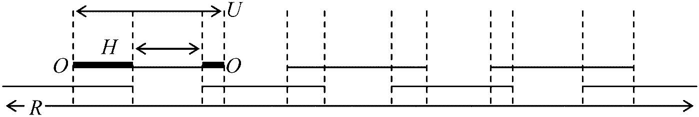 N = R/U·(1 + O–/H–) N: species richness, R: total resources, H–, averaged distance between the interrupted lines, C: number of neighboring species, R: range of resources, U: range of resources utilized by each species, O: overlaps of resource utilization R = Σi=1NHi = N·(1/N)Σi=1NHi = NH–∴ N = R/H– = R/U– = U–/H– → U– consists of two parts, H and O Σi=1NUi = Σi=1NHi + 2Σi=1N–1Oi, i+1 → divided by N
U– = H– + 2O–: the values are different between the two edges l: Rayleigh quotient on matrix α, α-: averaged competition coefficient, C: number of neighboring species |
Type 2: Evenness (均等度)Whittaker's evenness (Whittaker 1952)
Ec = S/(logp1 - logps)
S: species richness Bulla's evenness index, E (Bulla 1994, Feisinger et al. 1981)
E = (O - minO)/(1 - minO), D = Σi=1s{ni·(ni - 1)}/{N·(N - 1)}, or Σi=1spi → 1 - D
randamly selected one individual → Pi = ni/N, the probability that species i is selected Simpson's reciprocal index, 1/D = 1/Σi=1spi
→ non-sensitive to changes in species richness (becoming remarkable when species richness < 10 ↔ sentitive to the abundance of dominant species Phenological diversity, Df = 1/(eipi2) (→ Simpson) where pi is the relative frequency of each phenological group (in a given plot) Relative phenological diversity, D'f = (Df – Dfmin)/(Dfmax – Dfmin)
if phenological gropus are classified into four categories, then Evenness, J' = H'/H'max = H'/logS (Jost 2006, Tuomisto 2010) True diversity, qDγ (真の多様性)q (integer): called order of the diversity, qDγ ≡ (Σi=1spiq)1/(1 - q), q ≥ 0⇒ Hill numbers (effective number of species) q = 0: 0Dγ = Σi=1spi0 = sq = 1: 1Dγ = limq→11Dγ = exp(-Σi=1s(pi·lnpi)) = exp(H') q = 2: 2Dγ = 1/(Σi=1spi2) Table 1. Conversion of common indices to true diversities (Jost et al. 2006) Species richness x ≡ Σi=1spi0 x (diversity in terms of x)__Σi=1spi0 (diversity in terms of pi) Shannon entropy x ≡ - Σi=1spilnpiexp(x)________________ exp(-Σi=1spilnpi) Simposon concentration x ≡ Σi=1spi21/x___________________1/Σi=1spi2 Gini-Simposon index x ≡ 1 - Σi=1spi21/(1 - x)_______________1/Σi=1spi2 HCDT (or Tsallis) entropy x ≡ (1 - Σi=1spiq)/(q - 1)[(1 - (q - 1)x]1/(1 - q)______(Σi=1spiq)1/(1 - q) Renyi entropy x ≡ -ln(Σi=1spiq)/(q - 1)exp(x)________________(Σi=1spiq)1/(1 - q) Differentiating assemblages based on five compounds of diversity(Guisande et al. 2017) rarityheterogeneity (including species richness) evenness phylogenetic/taxonomic diversity, PD the sum of the lengths of all phylogenetic branches that are members of the corresponding minimum spanning path functional diversitycalculated by DER library in R Dark diversity= the set of species that are absent from a given site but present in the surrounding region and potentially able to inhabit particular ecological conditionsobserved community < species pool < regional richness ↑dispersal/habitat filtering/biotic interactions↑ |
 = between-habitat diversity
The species, population response within its niche hypervolume describes its niche. The amount of biotic change among units. The differentiation of units on the α-diversity scale is β-diversity Interspecific association and similarity between communities Qualitative data= binary data, or presence/absence dataMeasuring β-diversity with presence-absence data (Wilson & Shmida 1984)
H: given range of a habitat gradient
= association coefficient (Agrell 1945), faunistic relation factor (Webb 1950)
QS = 2a/(b + c + 2a)
SC = c/b (a ≥ b) PA = 1/2·(c/a + c/b) or c(a + b)/2ab Coefficient of closeness (親和係数), CC (Otuka 1936)CC = c/√(ab) Coefficient of difference (差異係数), CD (Savage 1960)CD = c/a (a > b) Kulezynsky similarity measure (カルチンスキー類似度), SM (Kulezynsky 1927)SM = c/(a + b - 2c) Debatable points (Southwood 1966)
Quantitative dataSimple correlation coefficient or Peason's φ (単純相関係数法) (Motomura 1935), or Product-moment correlation coefficient (積率相関係数), Cp (Goodall 1973)
φ= Σk(x1k - X1/n)·(x2k - X2/n)/[Σk(x1k - X1/n)2Σk(x2k - X2/n)2]1/2 |
Similarity ratio, SR (Janssen 1975)
SR = Σixi·yi/(Σixi2 + Σiyi2 - Σixi·yi) Percentage similarity, PS (Sorensen 1948)PS = 2·Σimin(xi, yi)/Σi(xi + yi) Percentage difference, PD (Odum 1950) or Bray-Curtis dissimilarity indexPD = Σi|Nai + Nbi|/(Na + Nb)
Na and Nb: total number of species in A and B, respectively
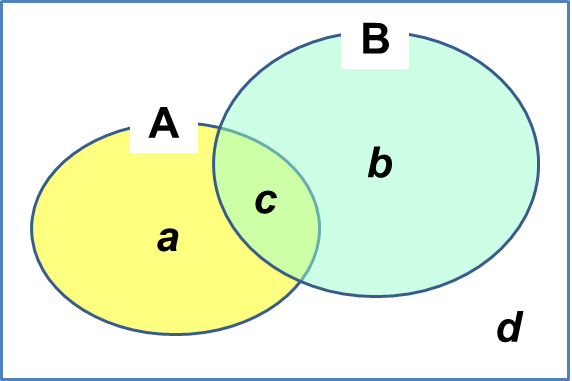
1 = completely different species composition between the two communities PS = 1 - 0.5·Σi|pai - pbi| = Σimin(pai, pbi) = Σmin(nx, ny)/(Nx + Ny) pai, pbi: dominance in communities A and B, respectively → application to succession (Tsuyuzaki 1991) Index of nichee overlap (S) (ニッチ重複指数)Coefficient of community, S1 = Σi=1min(pi, qi)Morisita's index, S2 = 2·Σi=1piqi/(Σpi2 + Σqi2) Horn's index, S3 = [Σi=1(pi + qi)log(pi + qi) – Σi=1pilogpi - Σi=1qilogqi]/(2·log2) Euclidean distance, S4 = 1 – [Σi=1(pi – qi)2/2]1/2Dissimilarity ⇔ Similarity (非類似度と類似度)C = a/(b + c + a) ⇒Def. Jaccard dissimirality, βdiss ≡ 1 - C
= 1 - a/(b + c + a) = {(b + c + a) - a)/(b + c + a) = (2 × c)/(a + 2 × c) when b ≥ c (∵ min(b, c) = c) (Villéger et al. 2014) Def. pturn ≡ βturnover/βdiss
= 2 × min(b, c)/(a + 2 × min(b, c)) × (b + c + a)/(b + c) Generalized dissimilarity modeling, GDM (一般化非類似度モデル)A statistical technique for modelling spatial variation in biodiversity between pairs of geographical locations or spatial patterns of turnover in community composition (β-diversity) (Library gdm in R package)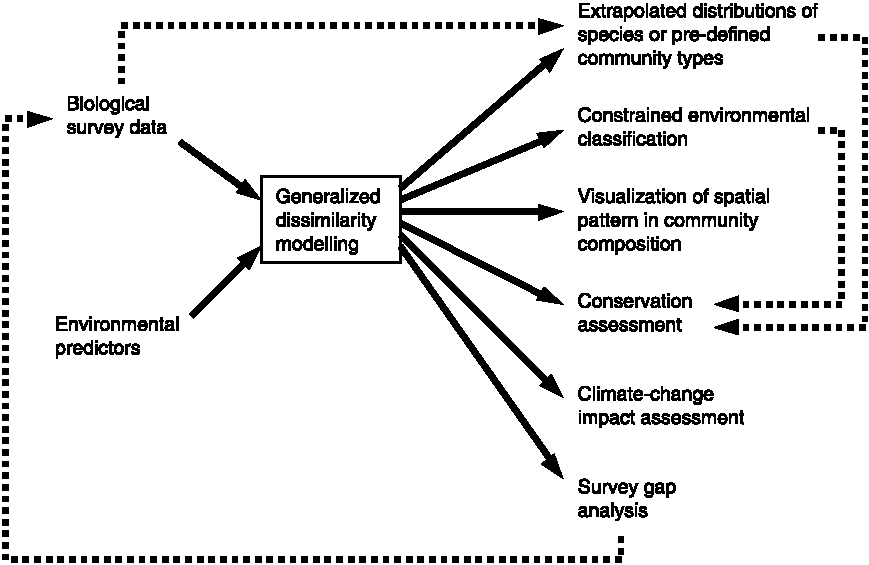 Fig. 5. Applications of generalized dissimilarity modelling Table 1. Approaches, utility, input data types, examples and associated software packages (Thomassen et al. 2010)
Canonical trend surface analysis: Modelling of biological variation across landscape |
| The variables of habitats and niches may be combined to define as axes an (m + m')-dimensional ecotope hyperspace. The part of this hyperspace to which a given species is adapted is its ecotope hypervolume. When a population measure is superimposed on this hypervolume, the ecotope of the species is described. |
Relationships between α, β and γ diversities(α, β, γ多様性間の関係)
    Community 1: A B C D E F
    Community 2:       D E F
    Community 3: A B     E F G
α1 = 6, α2 = 3, α3 = 5 (Veech et al. 2002, Baselga 2010) Additive partitioning: αavg + β = γβ = 7 - (6 + 3 + 5)/3 ≈ 2.33 Proportional partitioning: αavg × β = γ ⇐ β = γ/αavgβ = 7/{(6 + 3 + 5)/3} = 1.5 |
|
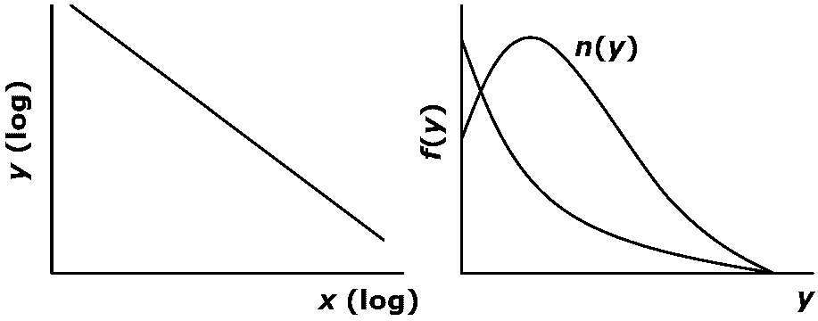
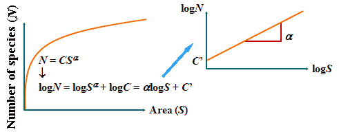
(Darlington 1957, Preston 1960) Species-area curve (種数-面積曲線)1921 Arrhenius O: linear log-log relationship between area and richnessN = CSα → logN = logC + αlogS
N: species richness |
|
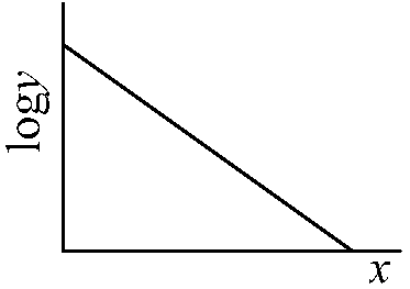
Zipf's law (ジップの法則)the law on the relationships between rank and size
Ex.1: 1897 Paleto: income of individuals Rank-size relationx: rank (in decreasing order of size y)y: size = Y(x) Size distriubtion function
the ratio of size that ranges between y and y + dy N: total number of species
f(y)dy = -d/dy·Y-1(y)dy
y ∝ x-(1 + α), logx + αlogy = C
y ∝ rx (r < 1), x + logy = C |
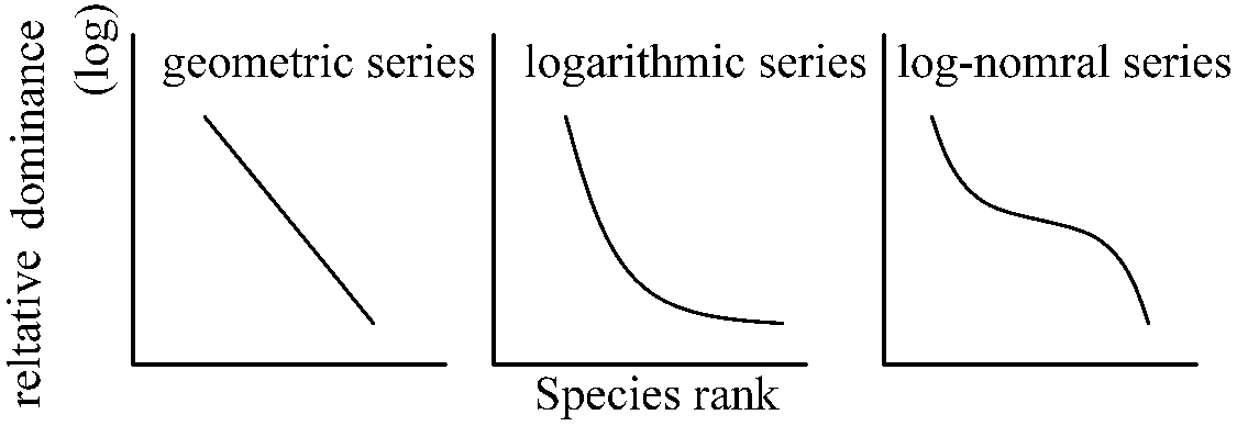
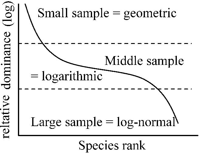
Species-dominance curves (種優占度曲線)→ x = rank and y = relative dominance on Zipf's law
S = aN - αN2, E = bN - βN2 a, α, b, β: constants dN/dt = r(1 - N/K)N → diversification curve K: constant, r = a - b |