(Upload on February 15 2018) [ 日本語 | English ]
Mount Usu / Sarobetsu post-mined peatland
From left: Crater basin in 1986 and 2006. Cottongrass / Daylily
HOME > Lecture catalog / Research summary > Glossary > Animal physiology
[ metabolism ] Animal physiology is totally different from plant physiology!
Physiologyclarifying function, law and principle in living systemsPhysics (L. nature) + logy (logos) = Physiology Pathos (L. relating to suffering and to diseases) + logy = Pathology (病理学) Causality (因果律): P → QNeurobiology (神経生物学)Behavior → nervous system (神経系)Comparative neurobiology
Sensory physiology [Input] |
Mechanical effector (機械的/力学的効果器) Ex. skeleton, muscle, flagellum, cilium Animal metabolism (動物代謝)Native peptide (天然ペプチド)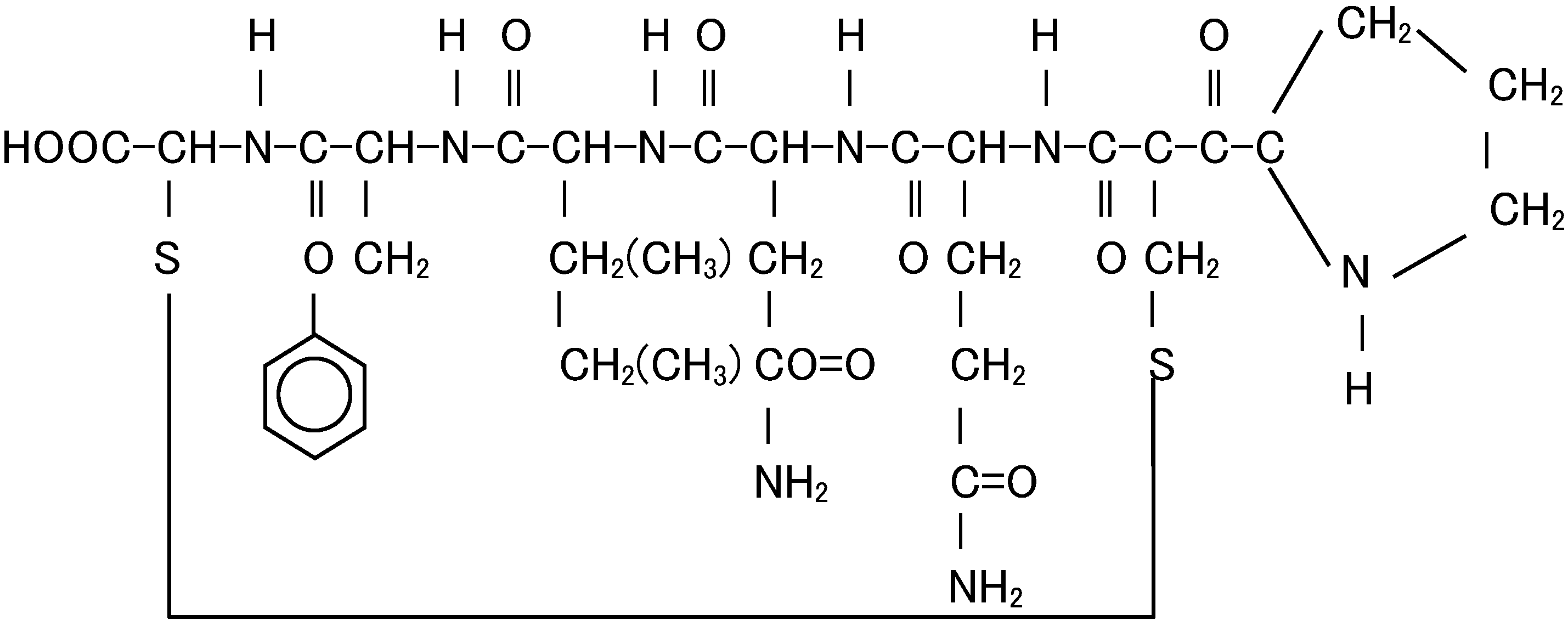 Fig. Structural formula of oxytocin (オキシトシン) |
|
Substance that acts in low concentration (μmol or less) Prodcued in one part of individual and act in another (translocatable) Has the same (or similar) response in many different species |
Muscle (筋肉)1934 Lohmann, Karl (1898-1978, German): Lohmann reaction
Creatine kinase (shuttle) Creatine kinase extracted a viscous protein from skeletal muscle of frog = myosin 1939 The Engelhardt: myosin = ATPase → called myosin-ATPasemyosin consists of two functional types of proteins Szent-Györgyi, Albert Nagyrápolti (1893-1986), Nobel Prize in 19371942 Szent-Györgyi: discovered two types of myosin Exp. extracted myosin from minced muscle by KCl
↓ a few hrs: extracted smooth myosin Sticky myosin: forming fibers by pushing the myosin in a syringe shrinkage by adding ATP = called active myosin (= actomyosin) Smooth myosin: no reaction with ATP = called inactive myosin 1942 Straub, Ferenc Brunó (1914-1996, working in Szent-Györgyi lab)discovered actin (separated from myosin) 1943 Straub: G-actin = monomer, F-actin = polymerG-actin polymerized into F-actin 1945 Straub: monomer (G-actin) containing ATP1945 Szent-Györgyi: reconstituted or synthetic actomyosin = functionally myosin B ⇒ natural actomyosin 1947 Szent-Györgyi: book entitled "Chemistry of muscular contraction"summarizing (actin + myosin + ATP = muscle movement) Natori Reiji (名取禮二) (1912-2006)1949 Natori: established skinned fiber method Huxley, Hugh Esmor (1924-2013) Hanson, Jean (1919-1973, England) 1953 Huxley HE & Hanson: determined proteins in muscles
A line: vanished by KCl solution cotaining ATP → myosin 1954 Huxley HE & Hanson: proposed "sliding filament theory" (滑り説) Myosin filaments slide into the gaps between actin filaments 1957 Huxley HE: determined the structure of muscle by EMHuxley, Andrew Fielding (1917-2012) 1957 Huxley AF: supported the theory by optical microscopic observation proposed a hyphthesis to explain sliding filament theory 1963 Hanson: structure of actin filament = double-stranded beads1966 Huxley AF: tension = myosine prominence-actin interaction 1972 Huxley HE: arrowhead structure of myosin aggregation Myosin molecules (ミオシン)1953 Cao (曹天欽): myosin treated by dense urea solutionsmall component of which MW is 20000 disassociated 1961 Takahashi K (高橋興威, 北大): myocine stained by negative staining1968 Lowey Susan: myocine molecule observed by EM both of them confirmed that myocine are two-headed with 150 nm l 1969 Stracker A: myosin treated by dense LiClseparated to H-chain (MW 2·105) and L-chain (2·104) → soon denatured 1969 Obinata T (大日方昂): chickensingle-head myosin in early development 1974 Maruyama K (丸山工作) et al.: cross-bridge model1976 Weeds AG: ATPase in L-chain operated by L-chain |
Actin molecules (アクチン)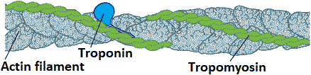 Fig. Tropomyosin (TM) binds to the side of adjacent actin subunits along the groove of the helix to stabilize and stiffen the actin filament. TM also prevents other proteins from accessing the filament. Troponin (actin monomer) controls the positioning of TM along the groove of the actin filament. F-actin binded with ATP vs G-actin binded with ADP 1962 Hayashi: F-actin → depolymerization → G-actin 1962 Asakura & Kasai (朝倉・葛西) polymerization rate ∝ (actin concentration)3 ⇒ trimer 1972 Gergely J lab. (Boston, USA): skeletal muscle of hare
determined the primary structure (amino acid sequene) of actin
∴ antibody to actin is not produced determined the polymerization is one-directional Calcium (カルシウム)1943 Kamada T (鎌田武雄): Ca-X → Ca + X, Ca → muscle contraction(later) X = endoplasmic reticulum 1948 Heilbrunn, Levis Victor: muscle fiber(+ calcium = muscle contraction) vs (+ ATP ≠ contraction) 1948 Bailey K: crystallized protein → tropomyosin1952 Heilbrunn: reject actomyosin-ATP system 1951 Marsh: predicted the presence of muscle relaxant factor (MRF) 1952 Bendall: demonstrated MRF + controlled (restricted) by calcium 1953 Szent-Györgyi, Andrew G (1924-2015): creatine kinase hypothesis 1955 Bendall: AMP-kinase hypothesis 1955 Kumagai, Ebashi & Takeda (熊谷・江橋・武田) Kielley-Meyerhof ATPase - relaxant action 1957 Roland: pyruvate kinase hypothesis1957 Portzehl H (disciple of Weber A) Kielley-Meyerhof ATPase presentt in microsome fraction 1964 Ebashi: active tropomyosin1965 Ebashi: troponin - binded strongly with calcium 1965 Makinose M (牧之瀬 望) & Hasselbach W active transportation of calcium uptaken by ATP
ATP + Ca2+ ⇄ Ca2EATP ⇄ EPCa2 ⇄ 2Ca2+ 1969 Smillie LB: determined amino acid sequene of β-tropomyocin 1972 Spring Harbor Symposium: unified the terminology of troponin
troponin C - calcium-binding component discovered by Gergely 1974 Gergely: steric-structure inhibition hypothesis Actinin (アクチニン)α-actininβ-actinin γ-actinin (Kuroda 1977) Euactinin (Kuroda & Mazaki 1980) Muscle proteinsM-proteinC-protein Z-protein |
[ human gastrointestinal system | digestive enzyme ]
Liver (肝臓)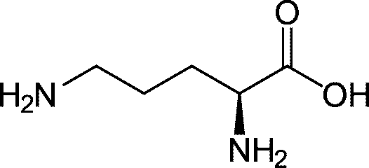 ornithine (Orn, オルニチン): C5H12N2O2 ornithine (Orn, オルニチン): C5H12N2O2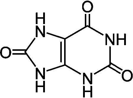 uric acid (UA, 尿酸)
 |
Ornithine cycle (オルニチン回路) Fig. Ornithine cycle. NAGS: N-acetylglutamate synthetase (EC 2.3.1.1; MIM 237310) CPS: carbamoyl phosphate synthetase (EC 6.3.4.16; MIM 237300) OTC: ornithine transcarbamylase (EC 2.1.3.3; MIM 311250) AS: argininosuccinate synthetase (EC 6.3.4.5; MIM 215700) AL: argininosuccinate lyase (EC 4.3.2.1; MIM 207900) Arginase (EC 3.5.3.1; MIM 207800) |
[ human urinary system ]
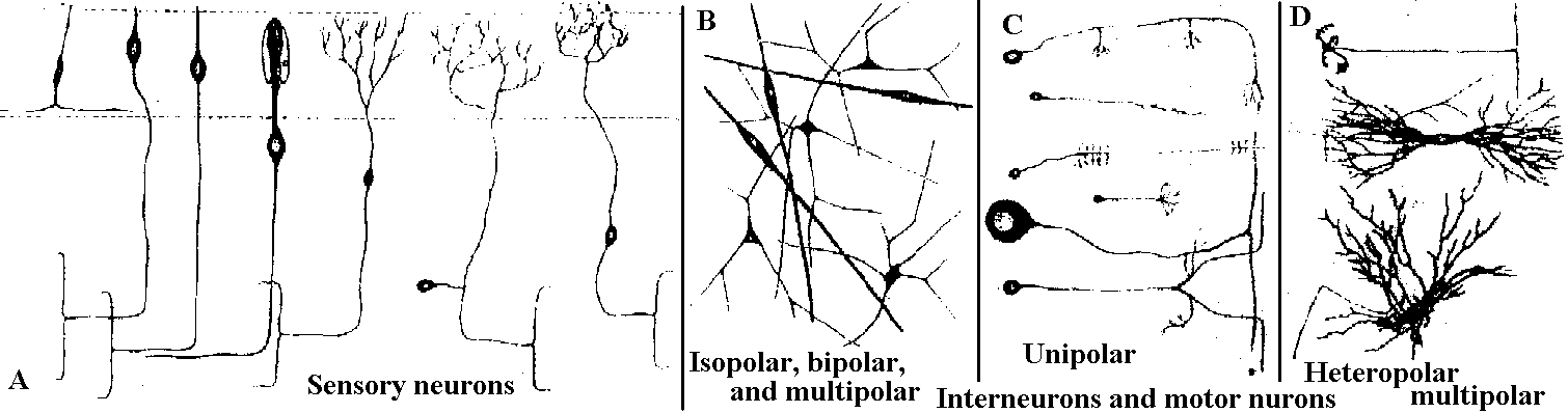
Fig. 2.1. Types of neurons, distinguished on the basis of number and differentiation of processes. A. Sensory neurons. The most primitive (far left) send axons into a superficial plexus. In animals with a central nervous system, the commonest form is a similar bipolar cell in the epithelium with a short, simple or slightly elaborated (arthropod scolopale) distal process and an axon entering the central nervous system and generally bifurcating into ascending and descending branches. A presumably more derived form (third from right) is that with a deep-lying cell body and a long, branching distal process with free nerve endings. In vertebrates, such cells secondarily become unipolar and form groups in the dorsal root ganglia. Shown on the far right is a vertebrate vestibular or acoustic sensory neuron that has retained the primitive bipolar form but has adopted (presumably secondarily) a specialized nonnervous epithelial cell as the actual receptor element. B. Isopolar, bipolar, and multipolar neurons in the nerve net of medusa. These may be either interneurons or motor neurons or both; no differentiated dendrites can be recognized. C. Unipolar neurons representative of the dominant type in all higher invertebrates. Both interneurons and motor neurons have this form. The upper four are examples of interneurons and the lower two of motor neurons. Afferent branches may be elaborate but are not readily distinguished from branching axonal terminals. The number and exact disposition of these two forms of endings and of major branches and collaterals are highly variable. D. Heteropolar, multipolar neurons-the dominant type in the central nervous system of vertebrates. The upper two are interneurons; the lower one, a motor neuron. (Bullock & Horridge 1965) 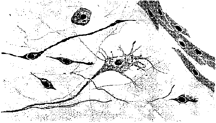 Fig. 7.13. Cells of the sponge Hippospongia impressed with silver. The central multipolar cell is regarded as a nerve cell centrifugal with respect to the cavity of a canal defined by a sphincter. (Pavans de Ceccatty 1959) 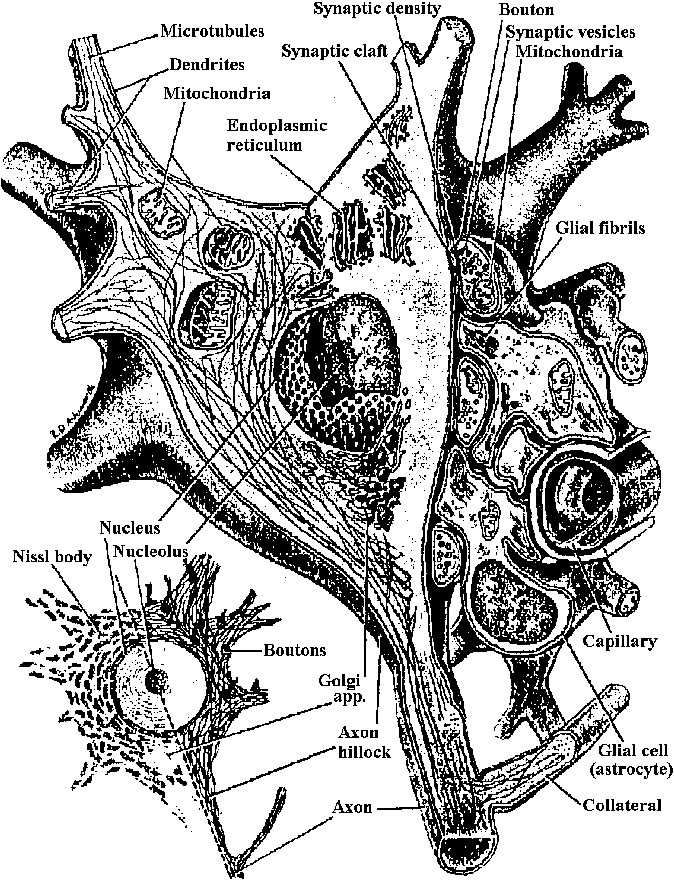 |
Figure 2.7. Nerve cell soma, showing organelles. The small view shows details seen at the light-microscope level. A stain selective for Nissl bodies was used on the left half; one selective for neurofibrils, on the right. The large diagram shows details seen at the electron-microscope level. (Willis & Grossman 1973) synapse シナプス nerve sheath 髄鞘 epineurium 神経鞘 Schwann シュバン核 Ranvier ランビエ紋輪 ganglion (pl. -a) 神経節 neurohumor 神経液 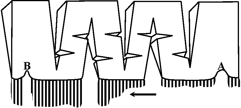 Fig. 3.9. The arrangement of classical experiment of Romanes, in which he showed the existence of two nerve net in the jellyfish Aurelia, and at the same time demonstrated a kind of reflex action rn the marginal ganglion. A part of the edge of the hell of the jellyfish is cut into a pattern such as that shown. The tentacles along the edge are allowed to relax. When tentacles at the right side in the region A are stimulated with a pinch, a wave of tentacle contraction spreads along the edge of the bell, although the excitation mtist obviously pass around the cuts, then this excitation reaches the ganglion shown at B, it initiates a tivave of contraction of the muscle. This second wave travels in the opposite direction around all the cuts with velocity of about 50 cm/sec, whereas the first wave travelled at only 25 cm/sec. Because the two waves have different velocities and cause different effects, there is strong circumstantial evidence for the existence of two nerve nets. In fact, two nets can be demonstrated by electrophysiological and by direct histologieal techniques. The wave of tentacle contraction can be compared with a sensory excitation and the wave of muscle contraction can be considered as a motor output of the ganglion. The interaction between these two kinds of excitation is always one-way in that the tentacle contraction excites the bell muscle excitation, so providing us with a primitive reflex arc. 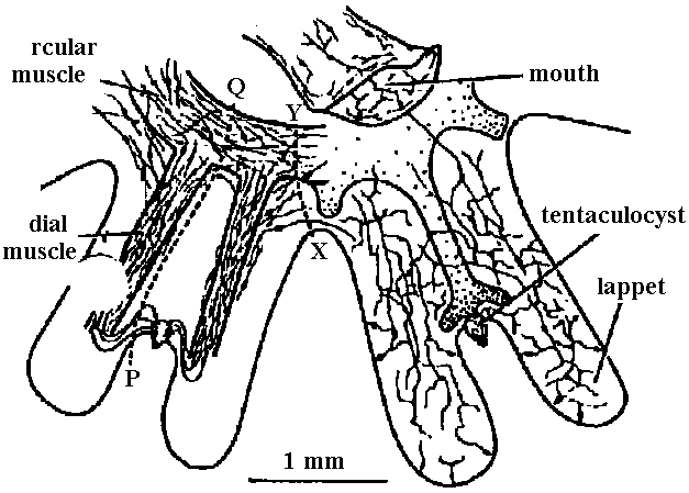 Fig. 3.10. One of the most primitive examples of differentiation between types of neurons, such that a neuron makes synaptic connexions indiscriminately with its own class of neuron but not with the other of the two classes. Two arms of the bell of the ephyra larva of the jellyfish Aurelia, showing the two t nerve nets, which can be stained with methylene blue. On the lef t are the muscle strips of the bell and the net of bipolar neurons, which coordinate them in the symmetrical swimming beat of the bell. The net of multipolar cells on the right connects with sensory cells and acts on the radial muscles in the local coordination of the feeding movements, in which one arm alone bends towards the month (Horridgc 1956) |
|
1. None 2. Diffuse nerve system (散在神経系): acceptor (受容体) → operator (作動体) 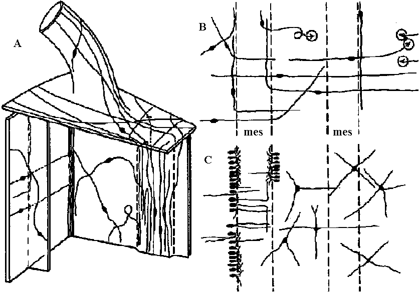 Fig. 3.7. Neuron pathways adjoining the mesenterices of anemones. A. Simplified innervation of portion of the anemone Mimetridum, showing individual bipolar neurons that run from body wall to mesenteries, from mesenteries to the ectoderm of the oral disc (via holes through the oral disc), and from oral disc to tentacle. The ectoderm of the tentacle is thus anatomically connected with the retraction system of the column, not only via the epithelium of the mouth. The presence of these bipolar cells sets a problem as to how the tentacles are coordinated without, spread of cxcitation to the column, implying a second conduction system in the disc. B. Bipolar neurons, similar to those in A, inside the column in the sphineter region of Calliactis. 'I'hc vcrticcal broken lines represent two mesenteries (mes) seen end on where they meet the outer wall. The bipolar axons pass around the body wall and through the mesenteries, as in A. C. Another system of cells superimposed on those of B. The unipolar cells are probably sensory. The multipolar neurons make connections with sensory and bipolar neurons. (A, Bathham 1965; B & C, Robson 1965) 3. Concentrated nerve system (集中神経系) Acceptor → central nerve system (integration, decision) → operator a. Ladder-like nervous system (梯子状神経系)= ganglionic nervous system (神経節神経系) 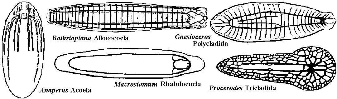 Fig. 9.1. Examples of the plan of the nervous system in representative turbellarians. (Left to right: Westblad 1949, Reisinger 1926, Hyman 1943, Lang 1881 & Hyman 1951) Ex. Basically, all the nerve system of insects is ladder-like 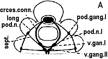
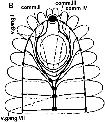 Fig. 14.7. A primitive and a more highly derived arrangement of circumesophageal nervous structures. A. Paramphinome. B. Hermodice (Gustafson 1930). crces. cann., circumesophageal connective; comm. II-IV. commissures of ventral ganglia II-IV; long. pod. n., longitudinal podial nerves (lateral nerve cord); pod. gong. I, first podial ganglion; pod. n.I, first podial nerve; sept., intersegmental septum; v. gang. I-II, first or second ventral ganglion. 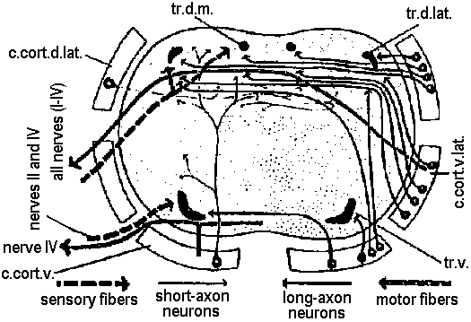 Figure 14.13. Diagrammatic transverse section of a nereid ganglion to show (1) the position of the long-axon longitudinal tract, (2) the directions of the long internuncial axons through the neuropile prior to their entry into the tracts, (3) the distribution of the short-axon internuncials, primarily confined in their collateral branchings to the dorsal neuropile, (4) the course and destination of the sensory fibers in fine-fiber longitudinal tracts, and (5) the course of the motor axons through the dorsal neuropile. The dorsal neuropile containing the greatest concentration of internuncial branchings is the more densely stippled (Smith 1957). c., cort. d.lot., dorsolateral sector of the cell cortex of the ganglion; c.cart. v., ventral sector; c.cart.v.lot., ventrolateral sector; tr. d. lot., dorsolateral. b. Tubular nervous system 管状神経系
Central nerve (integration, decision) → 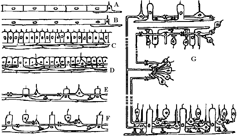 Fig. 4.8. The origin of the nerve cell. Hypothetical evolution of nerve nets in epithelial systems of ctenophores and coelenterates. A/B, conducting epithelium lending to nn epithclinl muscle cell. C, muscle cells connected by their tails. D, as in C, but with epithelial cells with processes that connect only with each other and bridge over intervening cells. This is the critical stage of appearance of axons, and there is no clue as to which type of cell gave rise to them. E, conacctions to muscle cells. F, origin of sensory cells, after the appearance of conducting systems. G, the situation in medusae and some other eoelenterates. There are 2 separate conducting systems, with separate sensory inputs and motor outputs; one system acts on the other at a definite place, as in the marginal ganglion in jellyfish. Invertebrate (無脊椎動物)Origin of neurons = epithalial cell (上皮細胞)
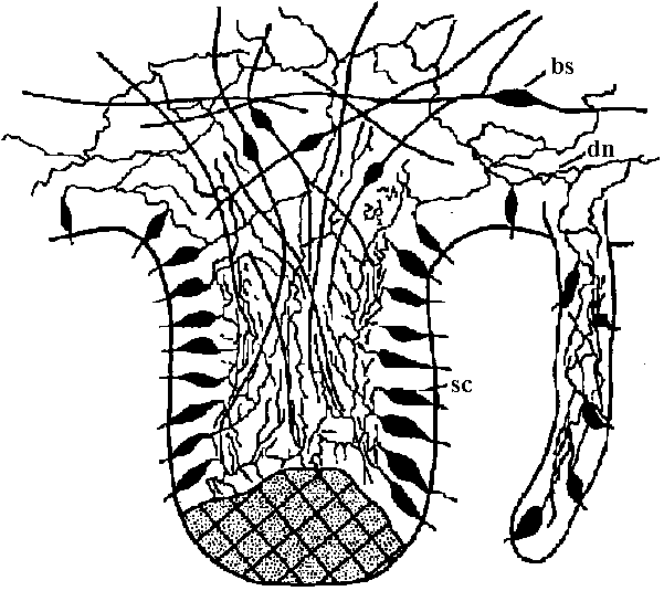 Fig. 3.11. Hypothetical organization of a jellyfish ganglion, showing the three main nervous structures that have so far been distinguished: the sensory cells of the ganglion (sc) the bipolar cells (双極細胞) of the motor nets (bs) with obvious contact synapses, and the difuse nerve net of the bell (dn), which has connexions with the other two neuron types in the ganglion. The shaded area represents the region of calcareous particles of the statolith. 
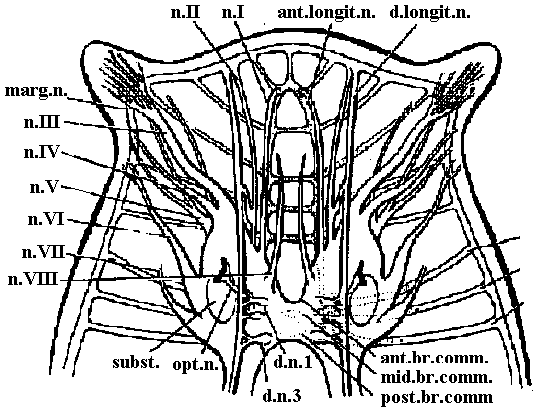 Fig. 9.6. Diagrams of the brain and anterior nerves. A. Geocentrophora baltica (Steinbock 1927). B. Planaria alpina (Micoletzky 1907). ant.br.comm., anterior brain commissure (接合部, 交連部); ant.longit.n., anterior longitudinal nerve; ant.v.n., anterior ventral nerve; cil.groove, ciliated groove; d.cord, dorsal cord; d.conn., dorsal connective; d.longit.n., dorsal longitudinal nerve; d.n.1 and d.n.3, dorsal nerve 1 and 3; lot.comm., lateral commissure; lat.cord., lateral longitudinal cord; lot. n. 1-3, lateral nerves 1-3; morg.n., marginal nerve; mid.br.comm., middle brain commissure; n.plex., peripheral nerve plexus; n. I-VIII, cerebral nerves 1-8; opt.n., optic nerve; post.br. comm., posterior brain commissure; ring comm., ring commissure; sens.nn., sensory nerves; subst., "Substanzinsel"; v.comm., ventral commissures; vlat.comm., ventrolateral commissures; viot.cord, ventrolateral cord. 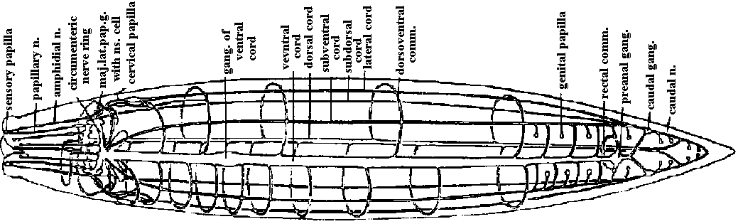 Fig. 11.8. Nematoda. Ascoris, plan of the nervous system, from the ventral side (Goldschmidt 1910, Voltzenlogel 1902). comm., commissure. gang., gangtion. moj.lot.pop.g. with ns.cell, ganglion of major lateral papillary nerve, with neurosecretory cell; n., nerve. Orthogon theory (or hypothesis) (直交体理論)A theory (or hypothesis) showing the develpment of basic nerve system
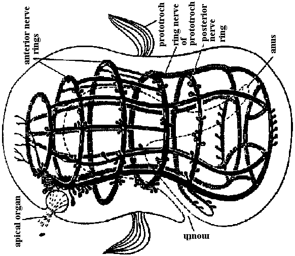 Fig. 14.1. Trochophore larva of Lopodorhynchus, showing the nervous system with its three nerve rings anterior to and one posterior to the prototroch nerve ring and its ciliated apical sense organ. (Hanstrom 1928) 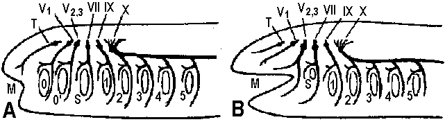 Fig. 380. Diagrams showing the distribution of branchial (dorsal root) cranial nerves. A, Hypothetic primitive condition, with typical nerves to each of two anterior gill slits lost in jawed vertebrates, and a terminal nerve to anterior end of head. B, Condition in jaw-bearing fishes. M, Mouth; 0, 0', anterior gill slits lost in gnathostomes; S. spiracular slit; T, terminal nerve; 1 to 5, typical gill slits of gnathostomes. VII: lower jaw, X, XI: visceral motor (smooth muscle, facial muscle – stricted muscle) 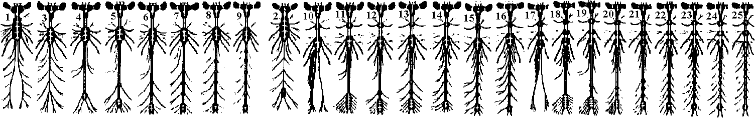 Fig. 16.38. The diversity of arrangement of ventral ganglia in various insects. 1 and 2 do not have a subesophageal ganglion: 3-9 have only one thoracic ganglion; 10-16 have two, and 17-25 three separate thoracic ganglia. 1, Hydrometrcs. Rhizotrogus; 2. Stylops: 3, Musca, Calliphoro, Lucilia, Sardophaga: 4, Ortalis, rrypeto, Conops, Myopa: 5, Syrphys, Volucella; 6, Cyrtus, Oncodes; 7, Stratiomys. Sargus, Haematopata; 8, Tabanus, Chrysops; 9, Panganha; 10, Bastrichus, Aecilius, Melalontha, Cetania; 11,Phora,Gyriflus; 12, Rhynchoenus; 13, Eucera, Crabro; 14, Vanessa, Pontia, Argynnis, Apis ♀♂, 15 Apis (♀♂), Bambus ♀♂, Andraena, Vespa (♀♂), Necrophorus; 16, Asilus, Tipulo, Culex, Bombus ♂, (♂♀), 17, Geotrupes, Aphodius, Areuchus; 18, Coccinello 5-punctota ♀. Scaphidium, Hister; 19, Harpolus. Chrysomela. Lmna; 20, Mutmlla rufipes ♂; 21, Mutilla eurapoea ♂. 22, Hepiahis, Sciara, Silpha; 23, Chiranamus. Cicindela, Blotto; 24, Telephorus. Lampyris ♀, Tenthreda, Sirex, Pulex ♀; 25, Pteronorcis. Dictyapterus, Pulex ♂. (Brandt 1878-1879) 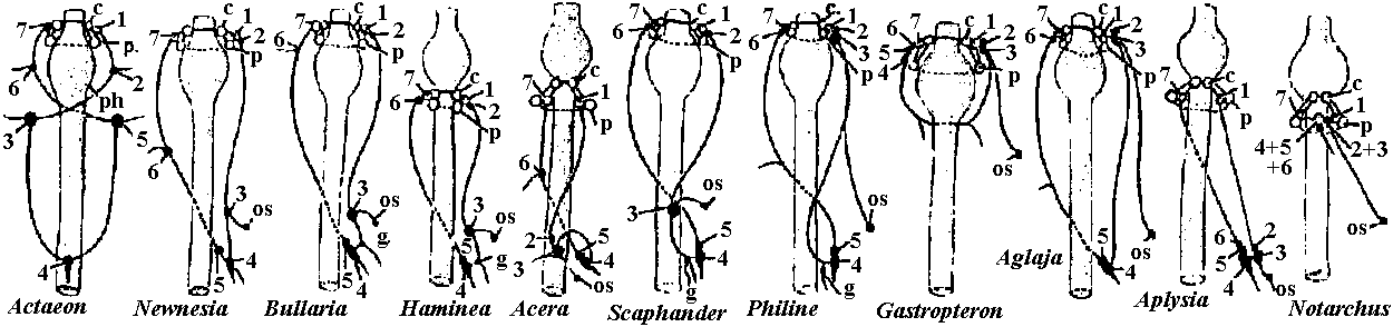 Fig. 23.63. Scheme of the principal forms of distribution of ganglia in cephalaspids (first nine genera) and anaspids (Aplysia and Notarchus) (Gulart 1901). c., cerebral ganglion; os., osphradium; p., pedal ganglion; ph., pharynx: 1 and 7, pleural ganglia; 2 and 6, parietal ganglia; 3 and 5, supra- and subintestinal ganglia; 4, visceral ganglion.  Fig. 16.32. Neurons of the ventral cord of the embryonic lobster, a, ascending interneurons with decussation; b, descending interneurons with decussation; c, two large descending interneurons from the brain and two smaller ones of the cord without decussation; d, abdominal motor axons having synapses between the symmetrical axons of the two sides; a, ascending and descending short interneurons with characteristic arrangement of synaptic contacts; f. examples of motoneurons with more than one axon, and other neurons described in the text; g, typical motoneurons; h, single neurons of the pairs shown in d, illustrating the units of which the pairs are composed. (Allen. 1894. 1896) 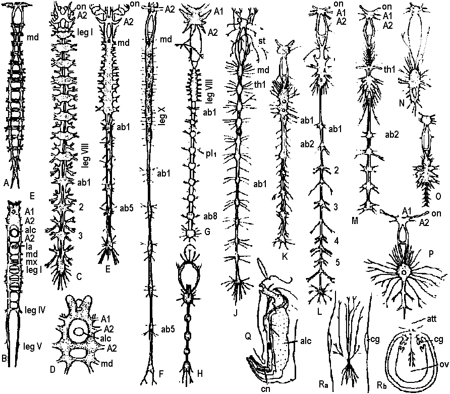 Fig. 16.26. Degrees of condensation of the ventral cord in some representative Crustacea. Since the anterior limit of the thorax is not sharply defined in many groups, the landmarks are mainly given with reference to the appendages. Most of these are taken from old figures in which smaller nerves were omitted. A. Anostraca, Branchipus venous (Hilton 1934). B. Cladocera, Simocephalus sima (Cunnlngton 1903). C. Amphipoda. Gammarus neglectus (Sars 1867). D. Cirripedia larva. nauplius of a pedunculate barnacle, showing the postoral second antennal region and commissure (Chun 1896). E. Mysidacea, Mysis relicta (Sars 1867). F. Euphausiacea, Euphausia superba (Zimmer. 1913). G. Stomatopoda, Squilla mantis (Giesbrecht 1913). H. Cirripedia, pedunculate barnacle (Hanstrom 1928). J. to P. Selected Decapoda (Balss 1944). J. Homarus. K. Pagurus. L. Paloemon. M. Golotheo. N. Palinurus. O. Parcellana. P. Carcmnus. Q. Parasitic Cirripedia, Acrothoracica, Cryptophialus (Berndt 1903). R. Parasitic Cirripedia. Rhizocephala, Peltagaster; (a) from ventral side, (b) transverse section (Delage 1886). ab 1, first abdominal ganglion; pl1, first pleopod nerve; th 1, first thoracic ganglion; Al, antennule nerve; A2. antenna nerve; alc., alimentary canal; att., attachment; cn, 6 nerves to cirri; cg, cement gland; la, labral nerve; md, mandible nerve; mx, first maxilla nerve; an, optic nerve; ov, ovary; st, roots of stomatogastric system. |
Neural structure of annelid (環形動物神経構造)
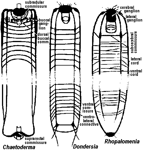 Fig. 22.2. Plan of the nervous system in Aplacophora three genera, showing degrees of regularity and completeness of the commissures (Wiren 1982, van Lummel 1930) 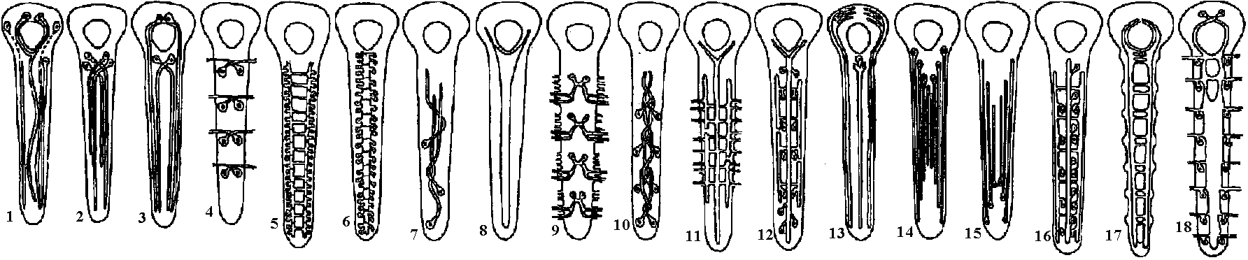 Fig. 6.6. Interneurons have evolved as giant fibres in a wide range of worms, usually acting as the fast pathways in general shortening of the body. Only one limitation is placed on the structure – that it be adequate. Even at this level there is no one-to-one relation between structure and response. 1-2, Euthalenessa; 3, Sigalion; 4, Lepidasthenia and Euthalenessa; 5-6, Lumbricus; 7, Euthalenessa; 8, Eunice; 9 and 10, Nereis and Neanthes; 11-12, Arenicola; 13, Nereis and Neanthcs; 14-15, Halla and Agiaurides; 16, Mastobranchlcs; 17 Sabella and Spirographis; 18, Myxicola (Nicol 1948) 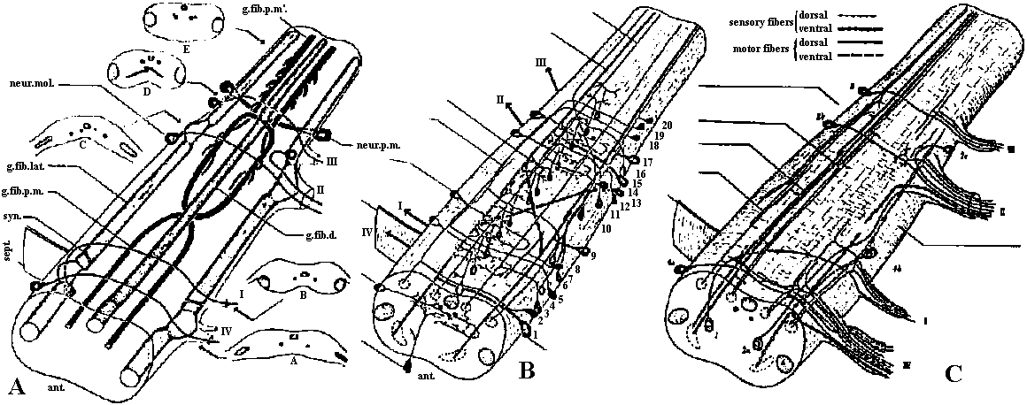 Fig. 17.11. Stereograms of a ganglion in the ventral nerve cord of the annelids Nereis diversicolor and Platynereis domerilii. The general arrangement of nerve cells in tile two species is similar. Imagine all three diagrams superimposed to gct an impression of the complexity of the organization of the annelid central nervous system. Four systems of neurons are shown: A, the giant neurons (giant fiber system); B, interneurons; C, sensory (fiber) and motoneurons. The nerve roots are indicated in roman numerals. The part of a septum (sept.) shown indicates the boundary between two body segments. There are five giant neurons: one dorsal (g.fib.d.), two paramedial (g.fib.p.m.), and two lateral (g.fib.lat.). The soma, or perikaryon, of the lateral giant fibers is not known, but these neurons are not longer than one segment: they form a wedge-shaped synapse (syn.) with the corresponding neuron of the next ganglion. The paramedial giants likewise reach only from one ganglion to the next; the two cross twice, then make synaptic contact with the corresponding cells in the next, anterior ganglion. The cell body or bodies of the dorsal giant fiber are situated in the subesophageal ganglion. This fiber runs uninterruptedly the whole length of the nerve cord. Certain motor neurons (neur.mot.) make synaptic contact with the lateral giant fibers. The neuropile is not shown in the diagrams. (Smith 1957) 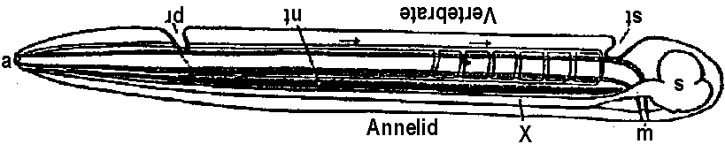 Fig. 11. Diagram to illustrate the supposed transformation of an annelid worm into a vertebrate. In normal position this represents the annelid with a "brain" (s) at the front end and a nerve cord (x) running along the underside of the body. The mouth (in) is on the underside of the animal, the anus (a) at the end of the tail; the blood stream (indicated by arrows) flows forward on the upper side of the body, back on the underside. Turn the book upside down and now we have the vertebrate, with nerve cord and blood streams reversed. But it is necessary to build a new mouth (st) and anus (pr) and close the old one; the worm really had no notochord (nt); and the supposed change is not as simple as it seems. Crayfish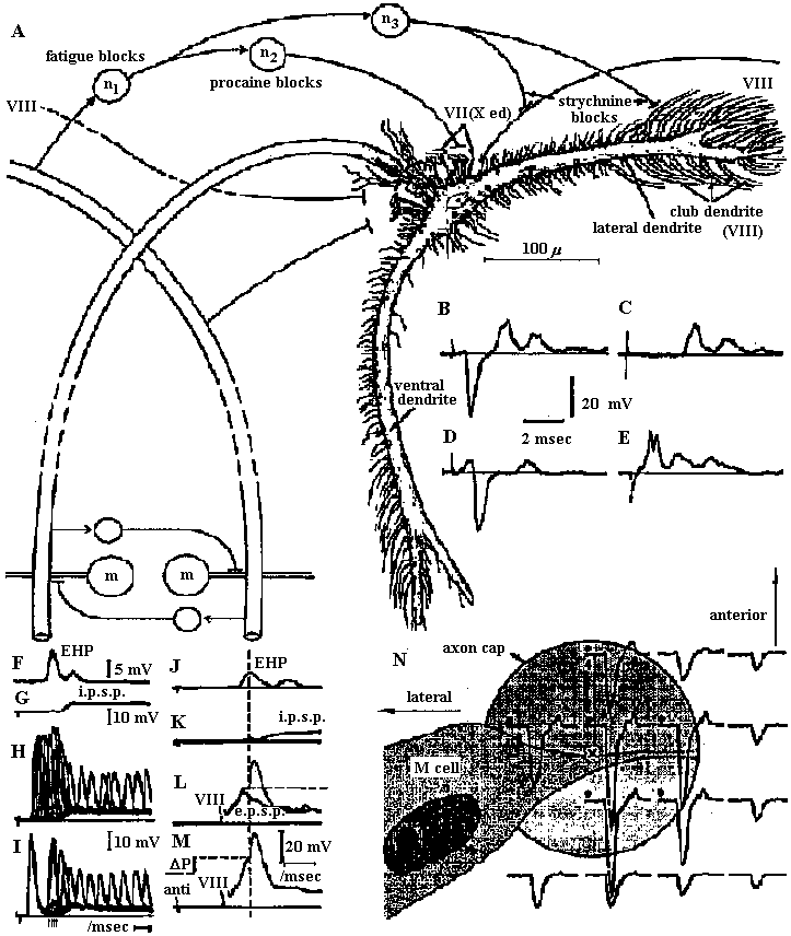 Fig. 5.9. Pathways of interaction between Mauthner neurons of the medulla of the goldfish, as inferred from extra-and intracellular records. A. The cell body of one side. The axon crosses its partner and runs down the spinal cord, where it forms synapses with motoneurons (m). The Mauthncr cell is normally excited primarily by the club endings from nerve VIII. Each Mauthner neuron inhibits the other by several intcrneuron pathtivays, which are distinguished by the action of drugs. The excitation of ni is blocked by fatigue and n2 by procaine. The presynaptic inhibition of n3, upon the fibres of nerve VIII is peculiar in being blocked by strychnine. The remarkable early inhibition is caused by extraccllular current in the region around the axon hillock (h). There is also an inhibitory pathway to the receptor. B-E. Comparison of extracellular potentials at one point close to the axon hillock under diff erent conditions. B. Both M cells are stimulated antidromieally in the spinal cord. C. Only the eontralnterul M cell is fired antidromicnlly. D. The ipsilateral M cell is fired by VIII nerve stimulation. E. Stimulation of the contraluteral VIII nerve. The ipsi- and contralateral M cells and stimulation of the contralateral VIII nerve each produces its own characteristie hyperpolurizing current. F-G. Simultaneous extra- and intracellular records, showing the extracellular hyperpolarizing potential (EHP) and the intracellular i.p.s.p., which is felt more strongly within the cell. H-I. Antidromic impulses (インパルス, 衝撃) superimposed ut different times on the i.p.s.p, are rcduced in amplitude. J-K. As in F-G, on a faster time scale. L. e.ps.p.'s generated by stimulation of the ipsilateral eighth nerve at diffcrent strengths (club ending pathways). M. Rasing the threshold to e.p.s.p.'s by ΔP as in L, by stimultaneous arrival of an EHP. This is the best indication of the inhibitory action of the extraccllular hyperpolarizing potential. N. Distribution of extracellular hyperpolarizing potential around the axon hillock of a Mauthner cell. The circle is 70 μm in diameter. (Modifications from Furukuwa) Mollusca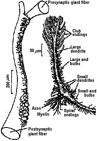 Fig. 2.17. Giant synapse in squid (Young 1939). Mauthner’s cell cynapse (Bodian 1952). 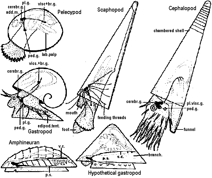 Fig. 22.1. Scheme of molluscan types, showing the plan of the nervous system. One ring around the gut is completed by the cerebral commissure above and pedal commissure below. The second is formed by the cerebro-pleural connective and the pleuro-visceral connective (or visceral loop or sling) and completed by the cerebral and the visceral commissures (or in place of the latter by the fusion into a single visceral ganglion). There is typically a pleuro-pedal connective but usually no direct connection between pedal and visceral (except in Amphineura) or cerebral and visceral. The gastropod shown is a prosobranch with torsion. The cephalopod is a tetrabranchiate with several kinds of tentacles (Naef 1928). add. in., adductor muscle; branch., ctenidia or gills; br. g., branchial ganglion; cerebr. g., cerebral ganglion; epipad. tent., epipodial tentacle; lab. paip, labial palp; ped. g., pedal ganglion; pl. g., pleural ganglion; p. s., pedal strand, a medullary cord not yet condensed into a ganglion; v. c., visceral cord or connective; visc. g.. visceral ganglion.
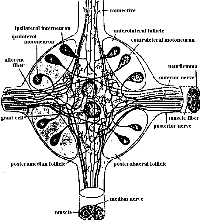 Fig. 14.19. Diagram of a typical ventral ganglion of a leech, showing the main nerve cells and fibers. At right and below, cross sections of the segmental nerve and the intersegmental connective, respectively. (Scriban & Autrum 1932) 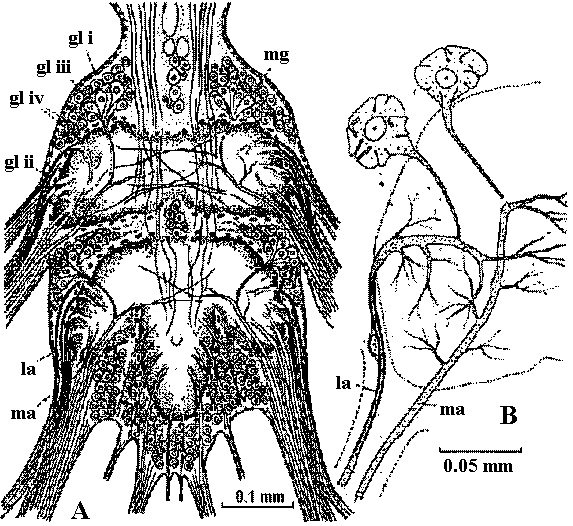 Fig. 17.10. A, diagram of the structure of a ganglion (fused mesotlsoracic, nsetathoracic, and abdominal ganglia) of the hemipteran insect Rhodnius, showing the relation of glia and nerve cells. Note the absence of cell bodies in the neuropile region. gl i, perineurium; gl ii, glial cells forming sheaths of lateral motor axons; gl iii, nucleus of giant glial cell; gi iv, nuclei of glial cells surrounding the dark neuropile; la, lateral motor axons; ma, medial motor axons; mg, motor ganglion cells. B, semischematic scale drawing of a typical lateral motor axon (la) and medial motor axon (ma). The dotted lines mark the boundaries of the nerve and of the dark neuropile. (Wigglesworth 1959) Fish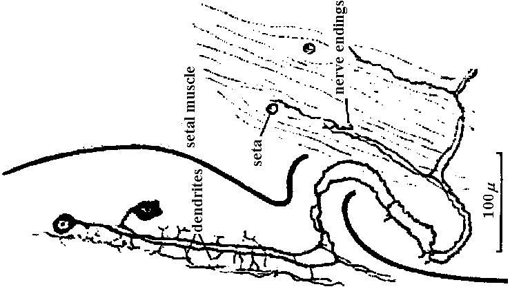 Fig. Two motoneurons to the muscles of the setae, in Pheretima, showing the manner of branching (Ogawa 1939) 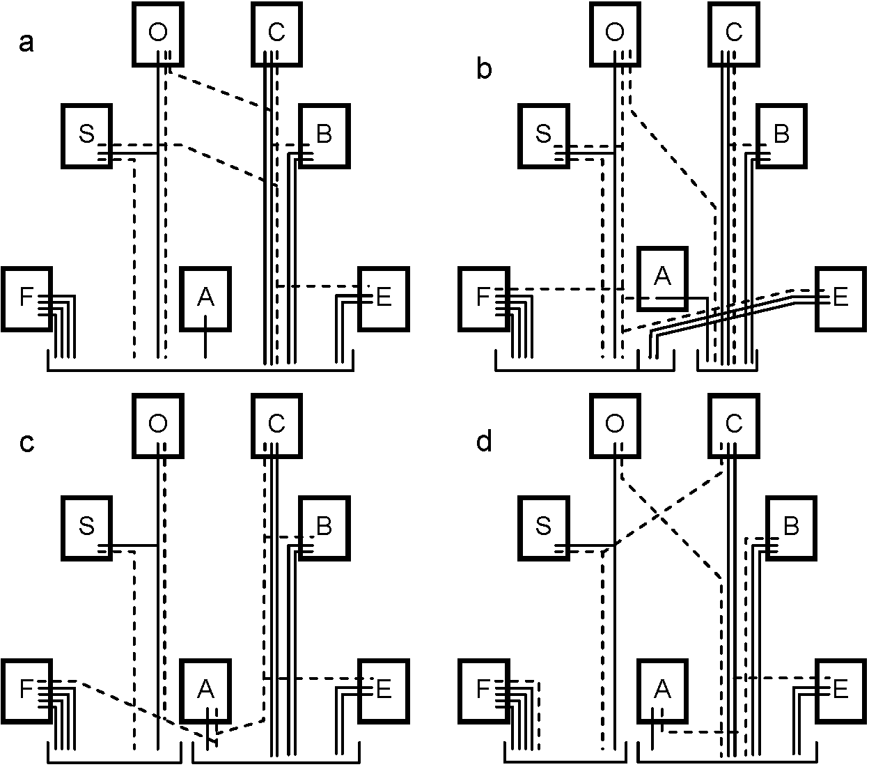 Fig. 24.9. Innervation schemas for the distal muscles in the thoracic limbs of the four Decapoda Reptantia tribes. a, Brachyura; b, Anomura; c, Palinura; d, Astacura. In the Anomura the common inhibitor is variable in position and may occur in the large nerve bundle. A, accessory flexor; B, bender; C, closer; E, extensor; F, main flexor; O, opener; S, stretcher. Solid lines represent single motor axons; broken lines, inhibitory axons; square brackets, distribution of axons between nerve bundles, the largest bundle being on the right. (Wiersma & Ripley 1952) |
|
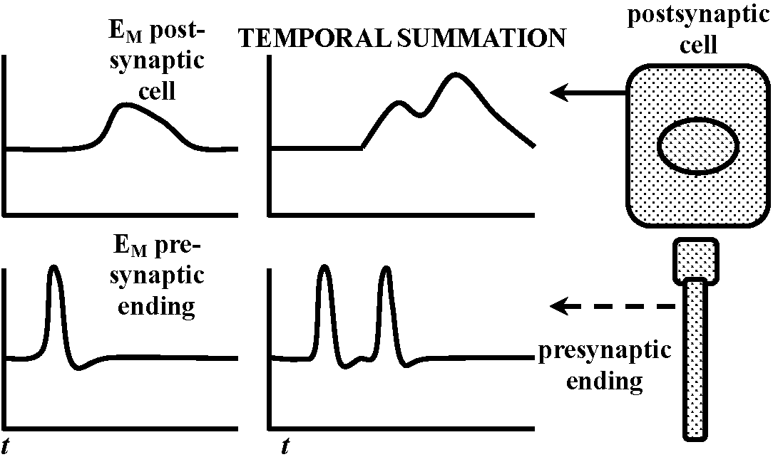 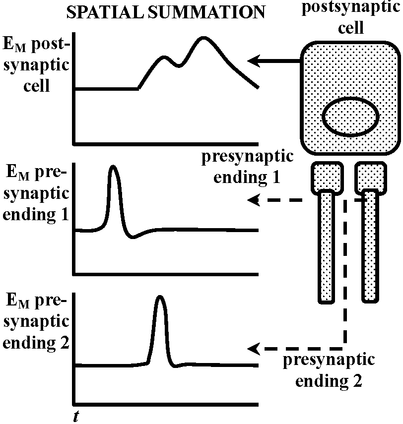 Fig. 20.33. Conceptual diagrams of temporal and spatial summation. 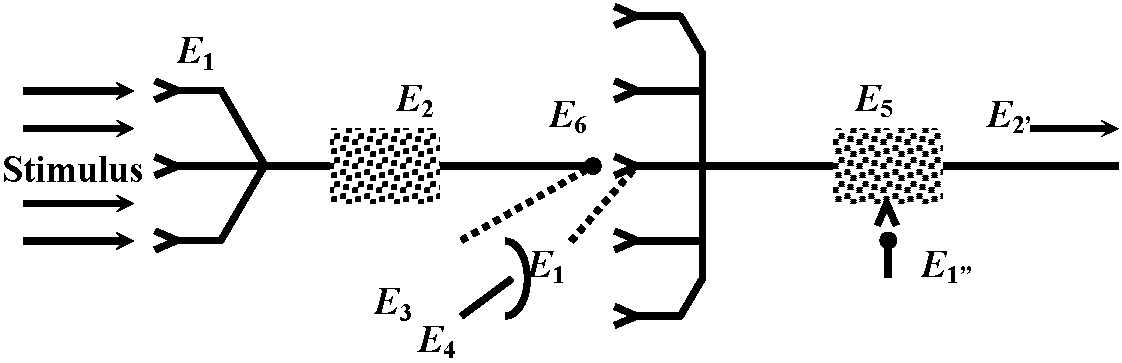 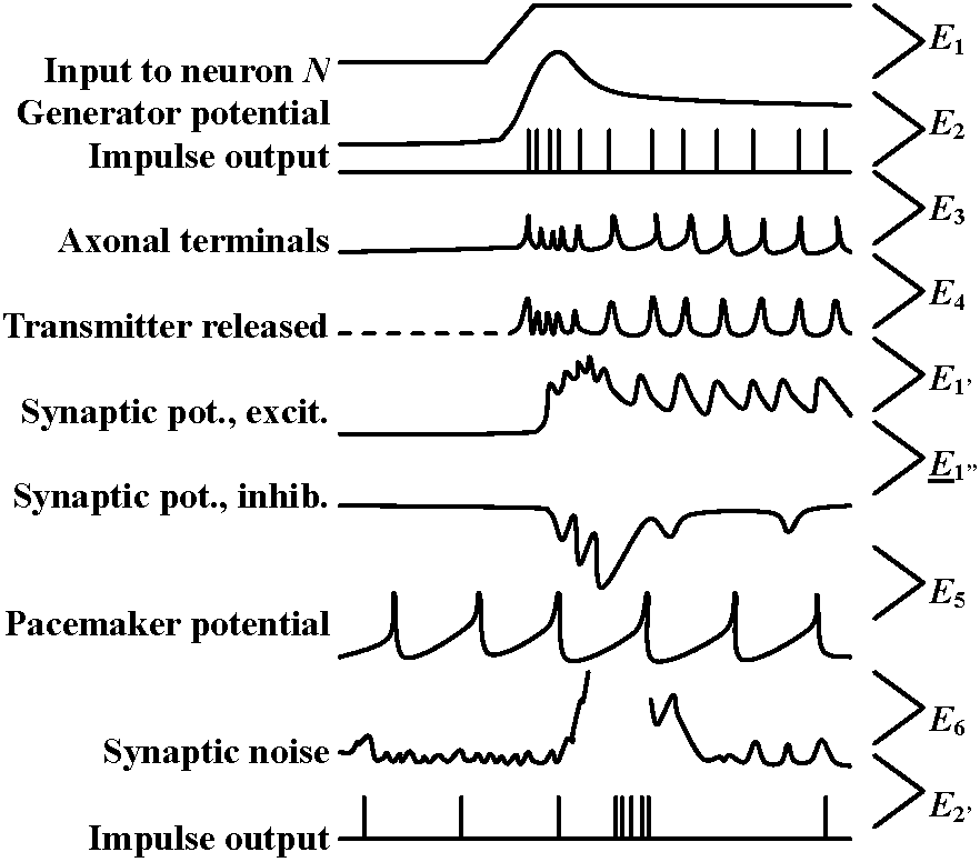 Fig. 6.2. Schematic diagram and summary of events plotted against time (ca 0.1 sec shown), showing several successive stages in the transfer of information from one nerve cell to another. The E's represent the independent excitabilities, or coupling functions, and the sites of possible molecular participation. The boxes in the schematic represent two nerve cells of order N and N+1; the synaptic contact between them is enlarged to show the L's involved. Release of transmitter is shown by a broken line, to indicate that the record is hypothetical. Broken leaders from some of the records indicate that the event just above that E is not the input for that E. (Bullock 1968) |
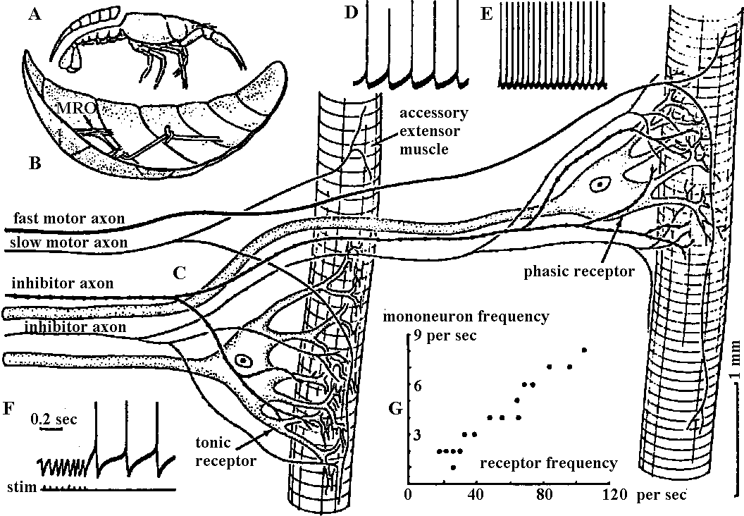 Fig. 6.1. One of the pairs of muscle receptor organs (MRO) of the crayfish or lobster, with tycpical responses. A. Removal of the dorsal side of the abdomen (Florey 1957). B. The boat-shaped preparation with one remaining accessory extensor muscle bearing a sensory neuron and other nerves (Florey 1957). C. The two modified slips of accessory extensor muscle from one side of one intersegmental joint as in B, showing the separate neurons. D. Typical intracellular response of the slow (tonic) receptor neuron to a small degree of stretch (Kuffler & Eyzaguirre 1955). E. The same, to a greater stretch (Kuffler & Eyzaguirre 1955). F. Suppression of activity by stimulation of the thick inhibitor axon at 20 per sec (Kuffler & Eyzaguirre 1955). G. The reflex relationship between the frequency of impulses in the tonic receptor and the impulses in a tonic extensor motoneuron of the same segment; that is, stretch of the sense organ causes a reflex contraction which relieves the stretch (Fields & Kennedy 1955). 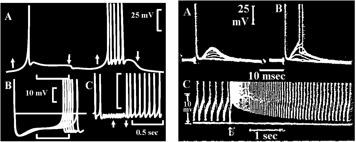 Fig. 18.15 (left). Intracellular recording from slowly adapting cells of the lobster. A. Receptor stretched and relaxed twince in succession. Time scale, 1 sec. B. Cell discharging at about 5 per second; each sweep is triggered by an impulse, so the prepotentials are superimosed. Time, 0.1 sec. C. The train of impulses is interrupted by simulation of the inhibitory axon at 34 per second; the small deflections are inhibitory potentials. Time, 0.5 sec. (Eyzaguirre & Kuffler 1955) Fig. 18.16 (right). Intracellular soma potentisals during contraction of receptor muscle of the crayfish. A. From phasic receptor cell. Motor stimuli at 4 per second with successive traces superimposed. Increasing twitches cause transient depolarizations reproducing the time course of the tension change. Each simulus also excites the sensory axon, which sends an impulse antidromically into the cell body, giving the first large deflection. B. At 10 per second the contractions reach threshold for discharge of the neuron. C. Augmentation of maintained discharge produced by two closely spaced motor stimuli (arrow) to the receptor muscle of the slowly adapting cell; contraction is relatively slow. Only the lower protions of the impulses can be seen (Eyzaguirre & Kuffler 1955) 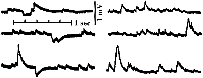 Fig. 20.28. Depolarizing and hyperpolarizing miniature potentials recorded from skeletal muscle fibers of the lobster (Homarus). The traces on the left were obtained from untreated fibers, those on the right from muscle fibers treated with picrotoxin, a drug that prevents the action of the inhibitory transmitter suhstance: note that the hyperpolarizing potentials disappear. (Grundfest 1961) |
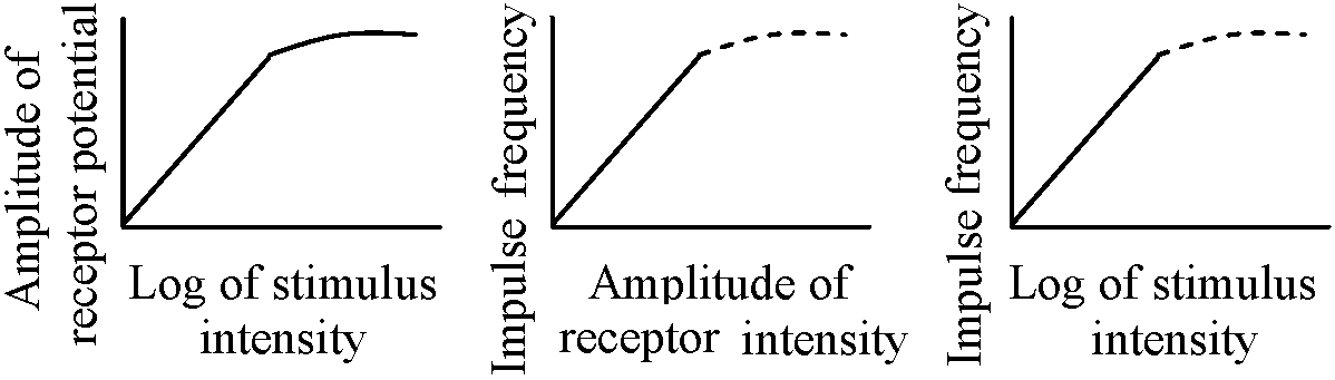
Receptor potentialStretch receptor (伸張受容器)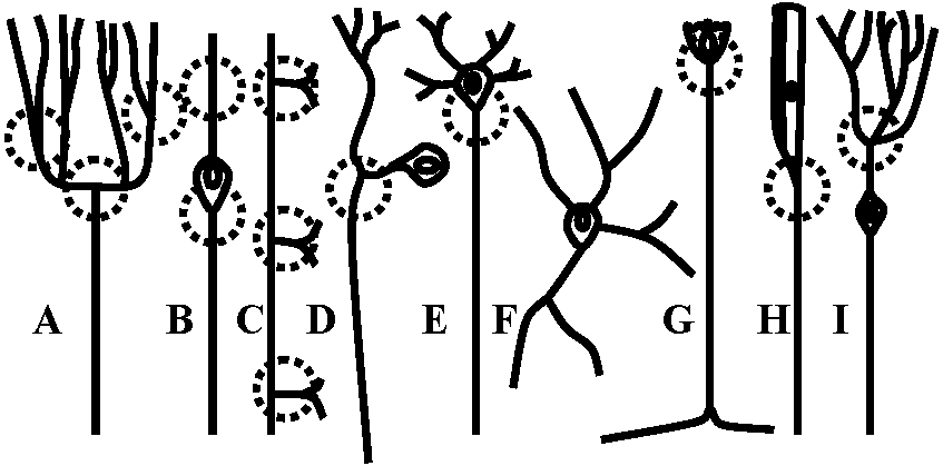 Fig. 5.4. The anatomical situations in which impulses are initiated. The dashed circles indicate the probable region where neurons of these varied forms have electrically excitable regions of lowest threshold. Neurons with sheaths that have nodes of Ranvicr can initiate impulses at the first or second node from the sensitive terminals A. Vcrtebrate sensory arborization. B. Typical invertebrate sensory neuron. C. Interneuron from a ladderlike cord with input and output in every segment. D. Typical invertebrate motoncuron. E. Typical vertebrate motoneuron. F. Amacrine cell (アマクリン細胞/無軸索細胞), or local interneuron, perhaps with no axon or spikes. G. Stretch receptor cell of arthropod abdomen. H. Arthropod primary visual cell, with rhabdom. I. Invertebrate sensory cell as found in some annelid, molluse, and other instances 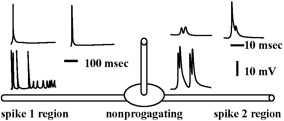 Figure 5.12. Two all-or-none spikes in one neuron. The intracellular recording electrode is within reception distance of two spike-initiating regions that must be separated by a nonpropagating region, as suggested in the diagram beneath. The records on the right are on a faster time scale. (Preston & Kennedy 1960) → observed becasue the central part of cell was stimulated 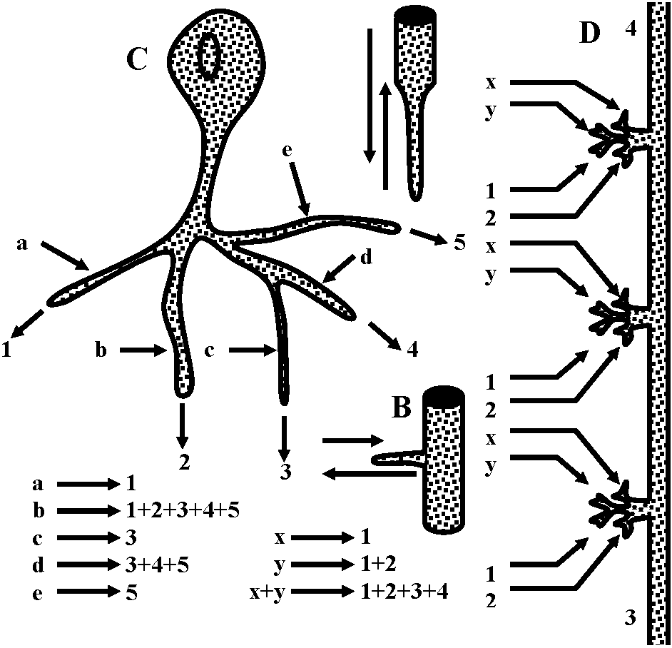 Figure 5.13. A swelling or a branching of an axon may reduce the safety fact.or for propagation of a spike to such a point that an integrating or polarizing junction is formed. A. A simpic swelling (for example the cell body of a bipolar neuron) can theoretically act as a junction with through-conduction in only one direction. B. The same at a side branch. C. Stimulation of different branches of one neuron, as in .Apli,.ia, can give rise to particular combinations of outputs as shown. D. An interacuron with arborizations in three successive ganglia in a ladderlike nerve cord. Inputs as shown by letters could give rise to outputs as shown by numbers. Because these relationships could be labile, as in synapses, the possibilities for modulation of an apparently stable anatomical pattern are extensive and as yet unknown. (C & D, Hughes 1965) 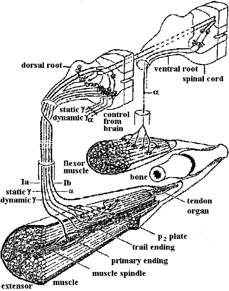 Fig. 175. Schematic diagram showing the location and innervation of a muscle spindle and a tendon organ in a cat ectensor muscle, and the synaptic connexions made in the spinal cord between their Ia and Ib afferent fibres and the alpha motoneurons innervating the synergic extensor) and antagonistic (flexor) muscles. Excitatory nerve cells and synaptic knobs drawn a open structures, inhibitory cells and knobs filled in. Ia and Ib pathways as postulated by Eccles (1957) Relationships between impulse frequencies and acceptors
Adaptation (受容器順応)
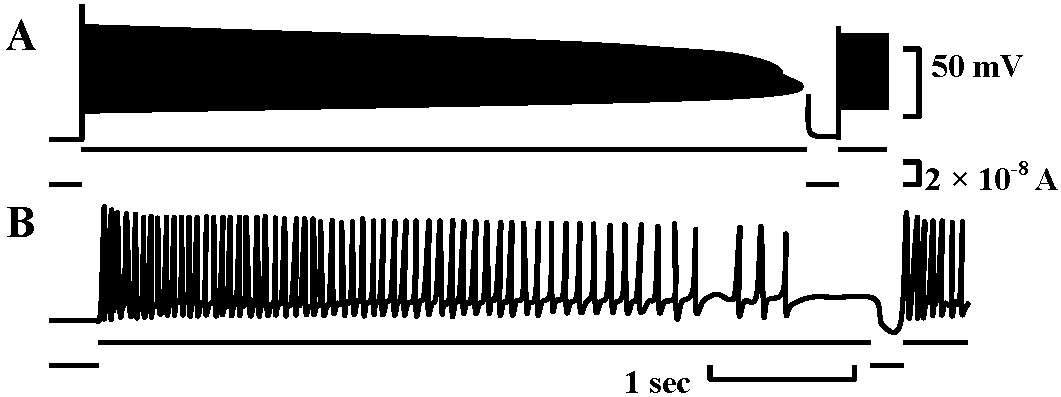 Adaptatio of spike initiation zone: Fig. 14. The behavior of spike adaptation elicited by intracellularly applied constant currents and the recovery from it by a short period of cessation of the current. A, a slowly adapting neurone stimulated by a strong constant current. When the spikes ceased, the current was turned off briefly. B, a rapidly adapting neurone. The applied current was smaller than in A. (Nakajima & Onodera 1969) 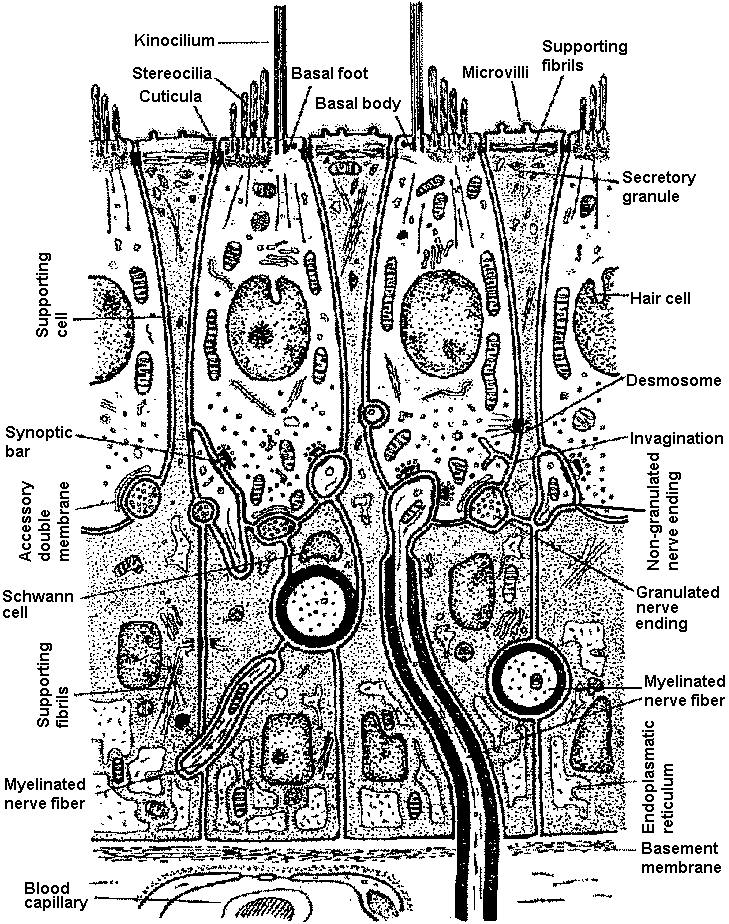 Fig. 4. Schcematic drawing showing the ultrastructure of the sensory epithelium of the lateral line canal organ of Lota vulgaris.
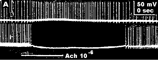
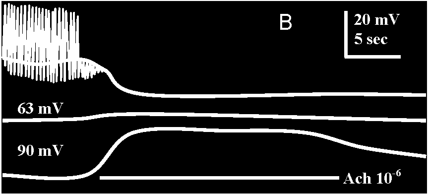 Fig. 20-31. A, simultaneous intracellular recordings from two contiguous and spontaneously firing D and H cells perfused with acetylcholine (ACh), 10-6 gm/ml, during the time indicated by the horizontal white line. B, action of Ach on a 11 cell which fires spontaneously and shows inhibitory posttsynaptic potetitials (i.p.s.p.'s), resulting from activity of a spontaneously active inhibotory neuron (like cell A in Fig. 20-30). Three superimposed records are shown. The upper one was taken under normal conditions; the average membrane potential is 40 mV. Ach causes hyperpolarization, cessation of spike discharage, and diminution of i.p.s.p.'s. The middle record was taken when the membrane potential was artificially raised to 63 mV. ACh now has no apparent effect, and the i.p.s.p.'s are no longer noticeable. The lower record was taken when the cell was artificially hyperpolarized to –93 mV. Under these circumustances the i.p.s.p.'s are larger. Ach causes depolarization and diminution of i.p.s.p.'s. The records demonstrate that the reversal potential of the i.p.s.p.'s is near –63 mV and that ACh shifts the membrane potential toward this value – evidence for the identity of the natural inhibitory transmitter with acetylcholine (Tane & Gersehenfeld 1962) 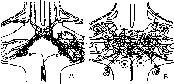 Fig. 20.5. Two diagrams representing the sensory (left) and motor (right) arborizations and branches which, together, form the neuropile. This is the core of the ganglion where the synaptic contacts are made between sensory and motor neurons and between cither of them and interneurons. The nerve cell bodies are situated in the periphery of the ganglion. This situation is typical of most invertebrate phyla. This figure represents the situation in a ganglion of the nerve cord of a larva of a (Dragonfly, Aeschna) (Zawarzin 1924) 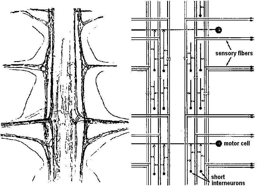 Fig. 6.7. Left: sensory tracts in the ventral cord of one segment of the earthworm, stained by the Golgi method. Where it enters the cord in a bundle in the segmental nerve, each sensory fiber divides and sends a branch in each direction. These branches combine to form long central sensory tracts (Rctzius 1892). This anatomical picture, together with the existence of impulses that appear to be efferent in sensory nerves, suggests that the sensors' axons stimulate each other in these central tracts, and that transmission along the tract occurs between terminals of primary sensors' cells, as illustrated on the right. Motor cells (large black circles) arc excited by inter-neurons (small unipolar cells) and possibly by the sensory tracts directly. Although the picture on the right shows an inferred plan so far as it is known in an annelid segmental ganglion, details must be extremely complex and different for each species. Nerve muscular junction (神経節接合部)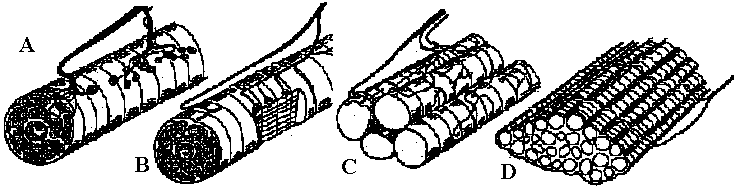 Fig. 2.20. Insect neuromuscular endings. A. The end-plate type; general in leg muscles of coleopterans and hymenopterans (also in the proboscis of dipterans; note fibril columns, mitochondria, and glial cell covering nerve ending with vesicles. B. The metameric type with circular end branches approximately between every two Z-bands; found in Dytiscus (Coleoptera) leg muscle. C. The diffuse type; general in Orthoptera; note fast and slow nerve fibers. D. The simple transverse type, with rarely ramifying circularly disposed end branches; genus in flight muscles of coleopterans and hymenopterans. Based on metallic impregnations and electron micrographs |
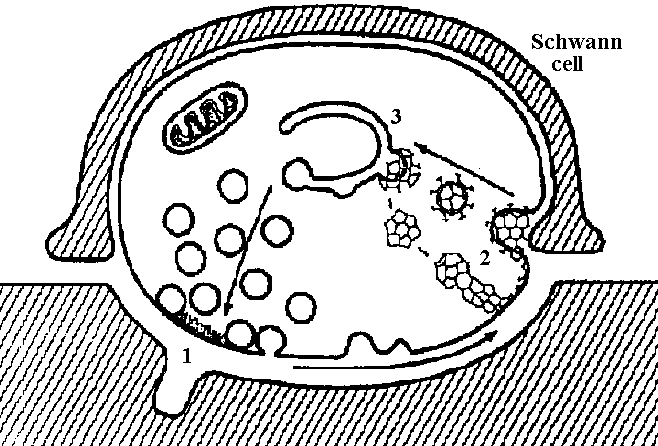 Fig. 5.11 Summary diagram of hypothesis for transmitter release at the neuromuscular junction, based on electron-microscopic observations. 1, vesicles coalesce with outer nerve terminal membrane and discharge their contents; 2, equal amounts of membrane are pinched off in region of Schwann cell and appear as coated vesicles; 3, coated vesicles then coalesce to form cisternae, which eventually reform new synaptic vesicles. (Heuser & Reese 1973) 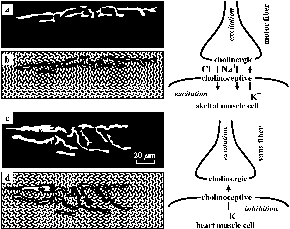 Fig. 20-29. Conceptual diagram of the action of acetyicholine as an excitatory as well as an inhibitory transmitter substance: in the case of vertebrate skeletal muscle, acetylcholine released from terminals of excited motoneurons increases the permeability of the subsynaptic membrane to chloride, sodium, and potassium ions, causing excitation. Acetylcholine released from excited vagus fibers inhibits the heart muscle cell by causing the subsynaptic membrane to become more permeable to potassium ion. The arrows show the predominant ion movement during transmitter action. (Florey 1962) Acetylcholine (アセチルコリン, Ach)= NMJ (neuro-muscular junction)Excitatory – heart muscle, peripheral blood vessel (表皮・筋肉系血管) Inhibotory – intestin (膜間), smooth muscle, blood vessel in internal organ (内臓系内部血管) 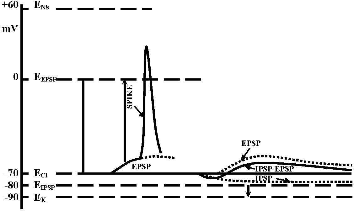
Em = RT/F·ln{ (PK [K+]o + PNa[Na]o + ···)/(PK[K+]i + PNa[Na]i + ···)} 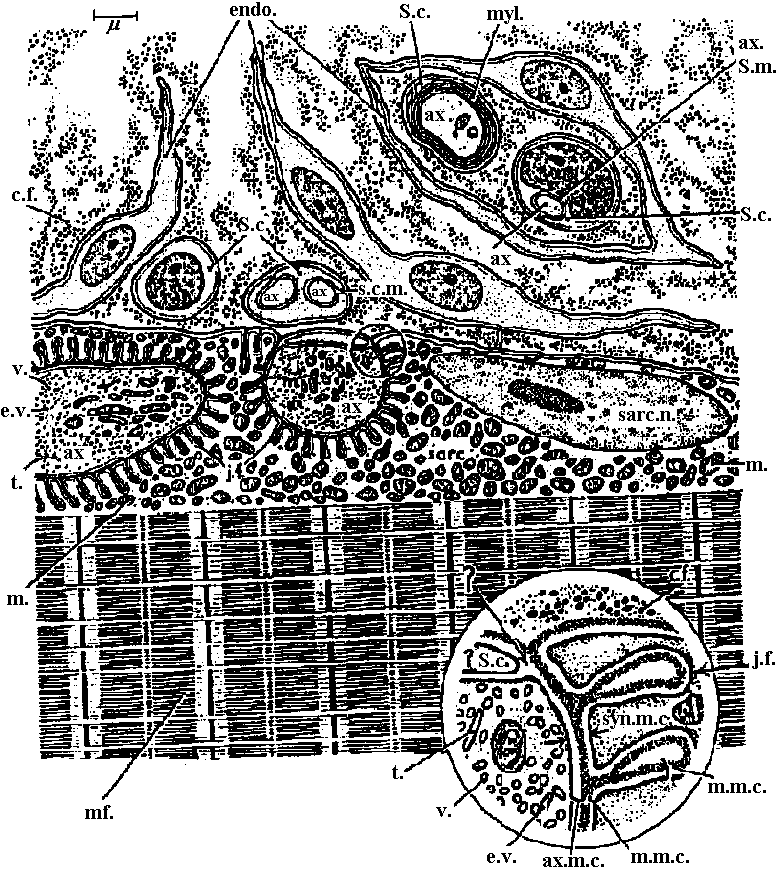 Figure 20.13. Diagrammatic representation of a neuromuscular junction on a striated skeletal muscle fiber of a reptile (Anolis). The diagram also shows (upper right quadrant) the axon (ax) of another motoneuron imbedded in a Schwann cell (S.c.) and surrounded by a cell of the endoneurium (endo.). Note the infolding of the sarcoplasmic membrane that surrounds (or almost surrounds) the motoneuron terminals. The latter are characterized by numerous vesicles (v.) and elongate vesicles (e.v.), as well as l)y many mitochondria (in.). Note also the numerous mitochondria in the vicinity of the synapse. Compare this diagram with the more abstract and schematic Figs 20-12; the latter does not show the endoneurial sheath cells. The region marked by the circle is shown enlarged in the lower right quadrant to show in more detail the junctional folds (j.f.), the muscle membrane complex (m.m.c.), and the nerve membrane complex (ax.m.c.). c.f., Collagen fibrils; mf., myofibrils; myl., myelin; sarc. n., sarcoplasmic nucleus; s.c.m., surface connecting membrane (= mesaxon); ax. S. in., axon Schwann membrane; t., tubule. (Robertson 1956) 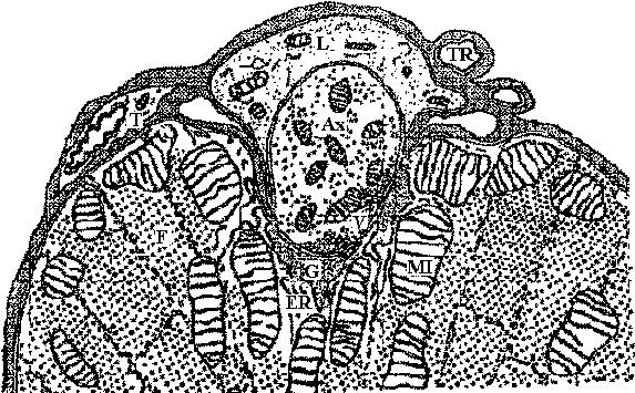 Fig. 20.14. Neuromuscular junction in a wasp leg. Note that it is completely enclosed. Tracheoles (Tr), with or without accompanying tracheoblast cytoplasm (T), are numerous in the contact region. The synapsing axon (Ax) in the muscle cell groove is essentially two-thirds covered externally by the lemnoblast (L). The basement membranes of the tracheoblast, lemnoblast, and muscle are merged. The final synapse involves apposition of the plasma membranes of axon and muscle fiber. The synaptic region is characterized by numerous mitochondria and synaptic vesicles (V) in the axon and by aggregates of mitochondria (ML), augmented endoplasmic reticulum (ER), and aposynaptic granules (C) in the muscle. In nonsynaptic regions the band-shaped myofibrils (F) and tubules of the reticulum are more regularly arranged (Edwards, Ruska & DeHerven 1958) Cholinergic transmission (end plate)Chlolinergic and adrenergic system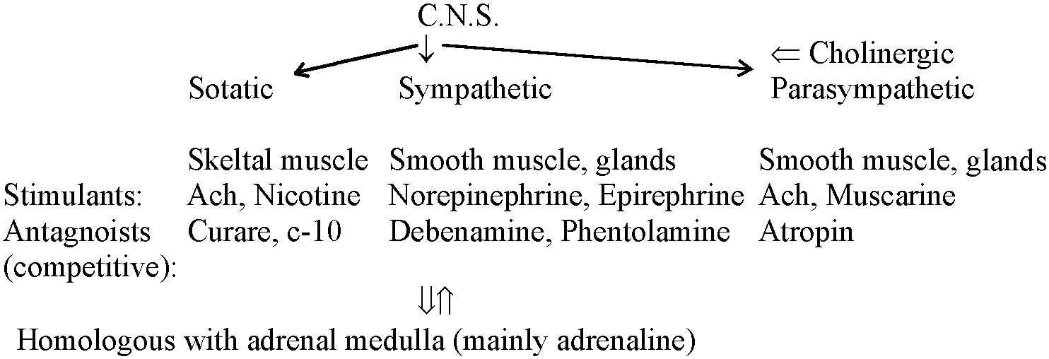
System junction = cholinergic, adrenergic Transmitter substances (伝達物質)EstablishedAcetylcholine (ACh): CH3-CO-COH2N(CH3)3
↔ Acetylcholine-like agents: carbachol, succinylcholine muscarine (ベニテングタケ) – activated in parasympathetic nerves → repaired by atropine ↔ Anticholinesterases (Acetylcholine-potentiating agents): eserine, neostigmine, edrophonium Norepinephrine (Noradrenaline): C6H10(OH)2-CHOH-CH2-NH2
↔ Noradrenaline-like agents γ-aminobutyric acid (GABA): COOH-CH2-CH2-CH2-NH2 Un-established DOPA: C6H10(OH)2-CH2-CH(COOH)-NH2 Dopamine (ドーパミン): C6H10(OH)2-CH2-CH2-NH2 octopamine: C6H11OH-CH(OH)-CH2-NH2 5-hydroxytryptamine (Serotonin) Glutamic acid: COOH-CH2-CH2-CH(COOH)-NH2 Energy transduction (エネルギー変換)Transduction (形質導入)Synapse (シナプス) = ganglion (神経節) 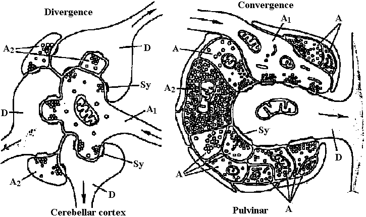 Fig. Two types of synaptic glomerulum. Complexes of synapses (Sy) involving several neurons seem to have evolved indendently many times. Some, as in the cerebellum, center on a single arriving axon minal (A); others, as in the pulvinar of the thalamus, center on a single depart dendrite (D) (Steiger 1967) 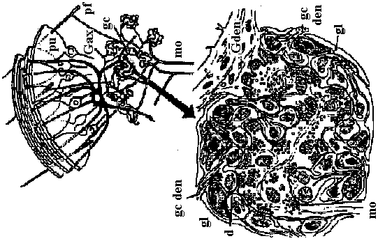 Figure 2.34. Synaptic glomeruli in the cerebellum. Above. A diagram at light-microscope mag showing seven glomeruli in the layer of granule eclls (gc). Below. One glomerulus EM magnification. tuc, mossy fiber afferents to the cortex; G ax (and shaded fiber) axon from Golgi cell (dark shading signifies an inhibitory influence, in this case to dendrites in the glomeruli); C den, Golgi cell dendrite; gc dcii, granule cell dendrit capsule; pf, parallel fiber granule cell axon; Pu, Purkinje cell; dd, desmosomoid de dendritic contacts. (Szentaothai, 1970)
= Post-synaptic potential e.p.s.p. (excitatory – p.s.p.) e.p.j.p. (excitatory – p.junction.p.)
depolarizing potential change – membrane worked towards depolarization direction 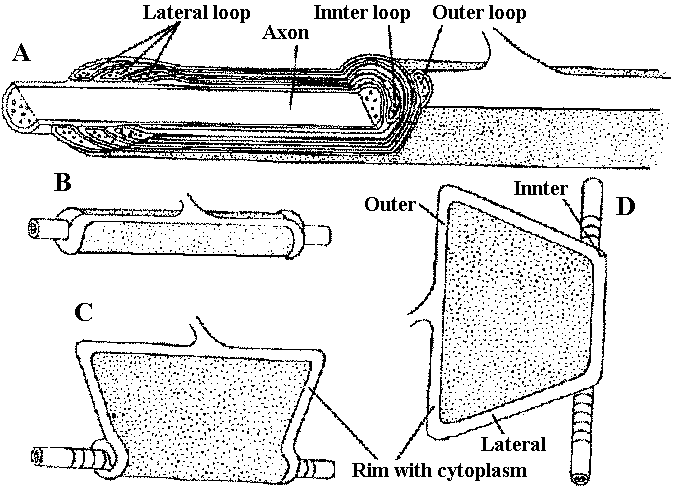 Fig. 2.47. The oligodendroglial myelin sheath of a single glial process, unrolled to show its structure (Hirano & Drebitzer 1967) 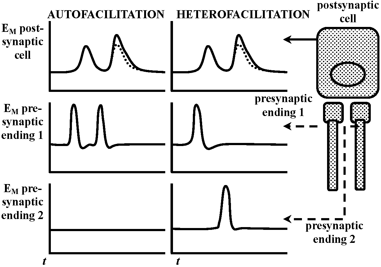 Fig. 20.35. Conceptual diagram of auto-and heterofacilitation. Note that when two presynaptic fibers are active, the postsynaptic responses to activity in each need not he ideutical. The responses indicated in stipple represent the response to the second impulse as it would occur in the absence of facilitation. |
Synapse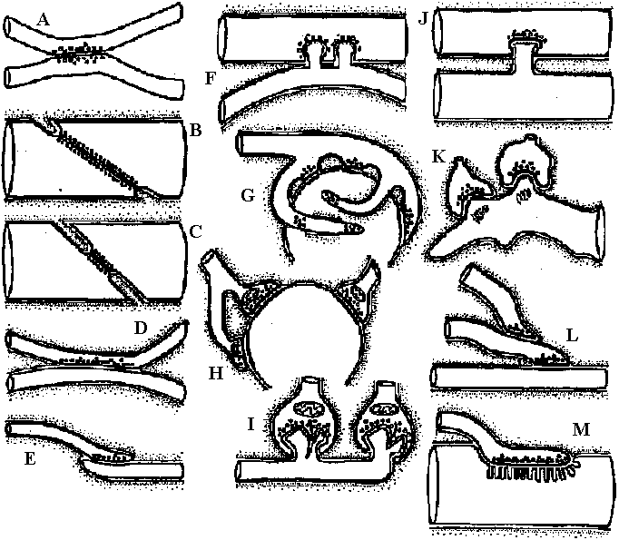 Fig. 2.27. Types of synapses revealed by electron microscopy. Brown, presynaptic; gray, postaynaptic; black, the lowermost extent of the sheath. A. Example of coelenterate axon-axon synapse in jellyfish ganglion, with vesicles on both sides and without adhering sheath cells. B. Earthworm septal synapse with close apposition of the membranes of the two cells and sparse vesicles on both sides. C. Crustacean septal synapse, as in B except that the synaptic area is restricted. Examples B and C have electrical transmission in either direction. D. Axon-axon synapse-in-passing typical of neuropile in many invertebrate ganglia, often with and often without sheaths. E. Axon terminal arborization ending on a fine dendrite in invertebrate neuropile. F. Crustacean giant-fiber-to-motor-neuron synapse, with postsynaptic motor fiber invaginated into the giant fiber. This example also has electrical transmission, but only in one direction. G. Axon arborization-to-soma synapse typical of vertebrate brain cells, but in invertebrates so far only clearly known as inhibitory endings on crustacean peripheral sensory cell of muscle receptor organ. H. Terminal buttons of axon arborizations typical of certain central neurons in vertebrates. I. Ribbon synapses between rod cell endings and dendrites of ganglion cells of vertebrate retina, with presynaptic specialization. J. Synapse between giant fibers of squid stellate ganglion, postsynaptic invaginated into presynaptic. K. Spine synapse (axon-dendrite) from cerebral cortical dendrite of vertebrates with postsynaptic specialization. L. Serial synapse, found so far in spinal cord, cerebral cortex, and plexiform layer of retina in vertebrates, but offering many potentialities for presynaptic inhibition and other complex interaction in neuropile. M. Specialized neuro-muscular endings found in vertebrate skeletal muscle, with postaynaptic grooves. (Bullock & Horridge 1965) 1909 Cajal: Dendrite law of dynamic polarity
– structural polarity (asymmetric tight junction)
|
observed without energization → reversal potential is -10mV Exp. 2: observed inhibiting post synaptic potential (i.p.s.p.) as the same way with Exp. 1 – cat spinal motoneuron
→ reversal potential is lower than the rest
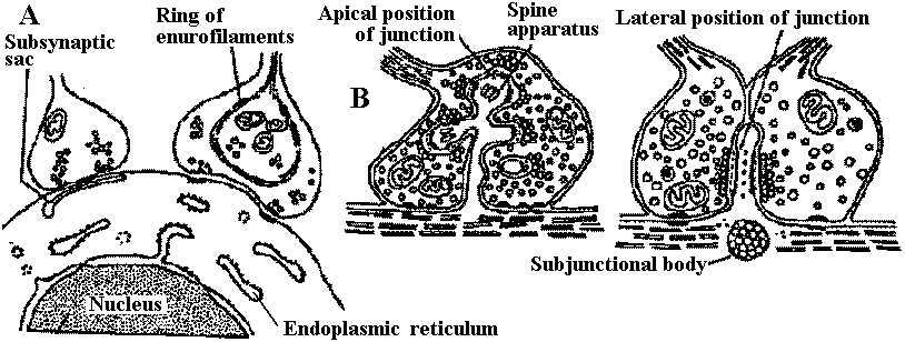 Fig. 2.31. Varieties of axosomatic and axodentritic synapses. A. Two subtypes of axosomatic synapse (Whitaker & Gray 1962). B. Two subtypes of axodendritic synapse (Hamlyn 1962) taxis (走性) |
Receptor (受容器)Exteroceptor (外部受容器)Enteroceptor (interoceptor, 内部受容器)
Proprioceptor (自己受容器): muscle spindle, stretch receptor (output monitor, feedback control) Phisical Exteroceptor Enteroceptor quantity Contact Distant
  Mechano-  Touch     Hearing           Propriceptor
                      Lateral line      Equillibrium receptor
                                        Carotid barroceptor
  Photo-    Taste     Vison             Carotid PO2, PCO2
                                        Chemoceptor
  Thermo-   Most      Pitorgan (snake)  Hypothalamie
                                        thermoceptor (視床下部)
  Electro-            Electroceptor
                      ↓ (latealline)
                      ↓ (loreziman oragan)
                      ↓ (ammpullary organ)
                      Model of synapse
Two types of sensory transduction
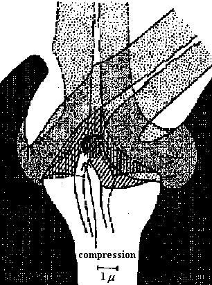
Primary sensory cell – Long distance transmission Mechano-receptors (機械受容器)contact of surface (skin, somatic sense) – touch (physical existence)sense of existence primitive and basic posture and position control – gravity (acceleration) vibration (substrate) - hearing medium (wind, kwater current, chemical, physical and thermal) responsible: electrical activity of sensory nerve 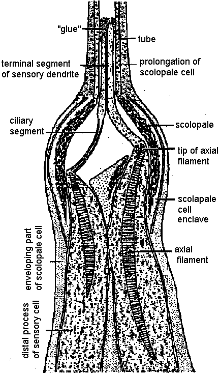 Figure 18.6. Complexity of a mechanoreceptor termination. Diagrammatic longitudinal section of a heterodynal scolopidium of the propodite-dactylopodite scolopophorous organ of Corcinus moenas, as revealed by electron microscope studies. The actual width of the figure is 3-6 μm. (Modified from Whitear 1960) 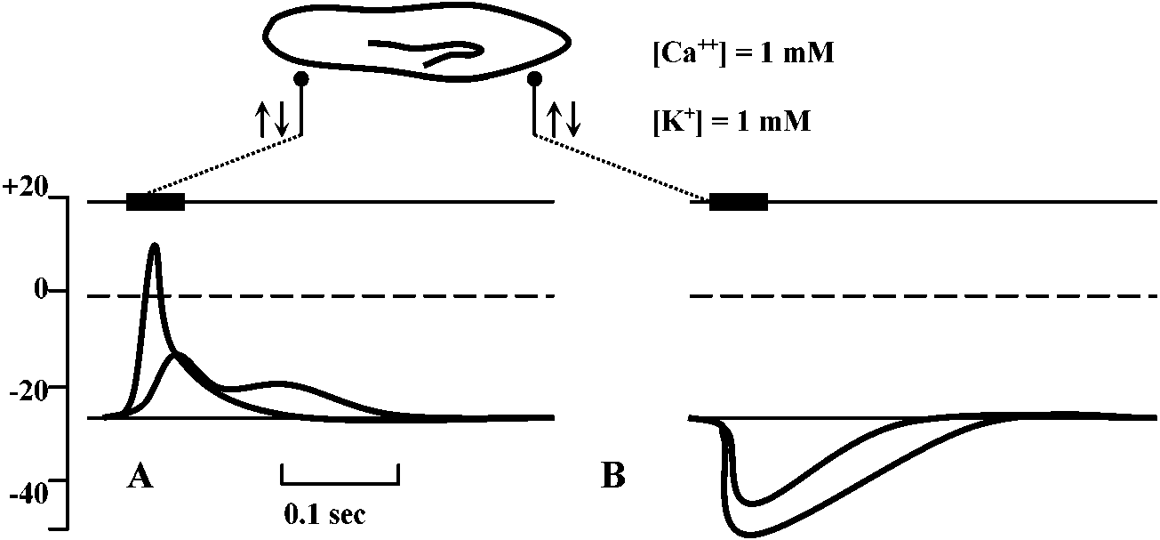 Fig. 1 (left). Mechanoreceptor potentials in Paransecium. Diagram shows an immobilized specimen impaled by an intracellular recording electrode. Mechanical stimuli of varying displacements were applied to either the anterior (a) or the posterior regions of the cell. (A) Anterior receptor potentials elicited by three intensities of mechanical stimulation of the anterior end. (B) Posterior receptor potentials elicited by mechanical stimulation of the posterior end. Deflections in the upper, trace show the duratioh and relative intensity of pulses activating the piezoelectric crystal. 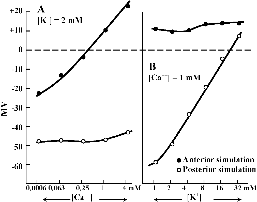 Fig. 2 (right). Peak values of receptor potentials plotted against Ca++ and K+ concentrations. (Ordinate) Intracellular potential recorded at the peak of the anterior receptor potential (○) and the posterior receptor potential (●). In graph A [K+] was held at 2 mmole/liter, and in graph B [Ca++] was held at 1 mmole/liter. Vertical bars show range of data from 5 to 12 measurements on as many different specimens. Only maximum responses were used. A maximum response was defined as one which shows no increase with further increase in stimulus intensity. 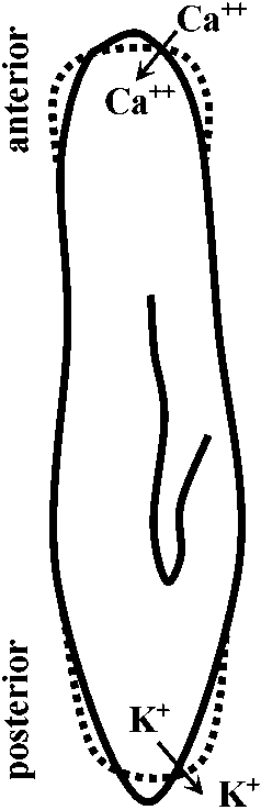 ↓ a) membrane deformation ↓ b) Ca++ permability increased ↓ c) Ca++ moves down electrochemical gradient ↓ d) potential approaches ECa: depolarization ↓ e) depolarization spreads electornically ↓ f) cilia reverse direction of beat ↓ g) reversed locomotion; avoiding reaction ↓ a') membrane deformation ↓ b') K+ permability increased ↓ c') K+ moves down electrochemical gradient ↓ d') potential approaches EK: hyperpolarization ↓ e') hyperpolarization spreads electornically ↓ f') beat frequency increased ↓ g') forward locomotion; avoiding reaction Fig. 3. Summary of steps linking mechanical stimuli with motor reactions of Paramecium. The anteiror and posterior ends of the organism are shown at the top and bottom, respectively. Major steps leading to either the avoiding raction or accelerated forward locomotion are outlined near the end of the cell which when stimulated initiates the sequence. The molecular mechanisms involved steps a, a’, f, and f’ are not known. 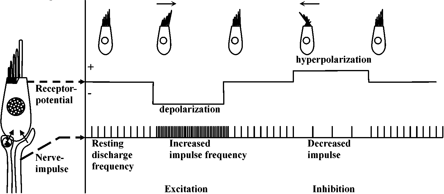 Fig. 14. Diagrammatic illustration of the proposed theory of hair cell function showing the relation between the receptor potential and the frequency of nerve impulses (インパルス, 衝撃) when the sensory hairs are inclined toward or away from the kinociliuin. 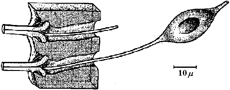 Fig. 1. Part of the hair-plate organ in the neck of a bee as it appears with methylene blue staining. The distal nerve process of a bipolar receptor cell enters the joint region of a hair through a canal in the cuticle. Frontal section in the axis of symmetry of the sensilla. (Thurm 1963)
hair sensilla (感覚毛) 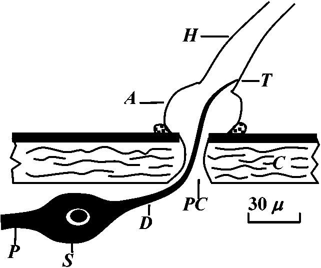 Fig. 25.11. Homarus: relationship between the statocyst hair and its single sensory neuron. The cell body (S) of the sensory neuron lies in the hypodermis surrounding; the statocyst and sends a distil process (D) through a pore canal (PC) in the cyst will (C) to enter the hair base and terminate in the region where pair shaft (H) joins the dilated (adj. 拡張した, 膨らませた) basal ampulla (A). A proximal (adj. 近接した, 基部に近い) procecc (P) runs to the brain in the statocyst nerve. The precise location and nature of the ncrve terminal junction (T) with the hair is not yet clear find this picture represents an approximation from thc bast available evidence. The drawing is to scale except thnt the distal nerve proccess may sometimes be as long as 500 μm. (Choen 1960)  Fig. 2.11. A largely hypothetical diagram of the pathways between sensory neurons, nerve net neurons, and muscle fibers in the finger of Lezccothea. This method of drawing out a theoretical explanation leads to further qualitative questions of stricture. The act of drawing it prompts such questions as the number and position of connections, the length of nerve and muscle fibres, the relative abundance of different cells, and the reality of the connections shown. The thicker nerve fibres show the system that is distinguished as that responding to vibration. 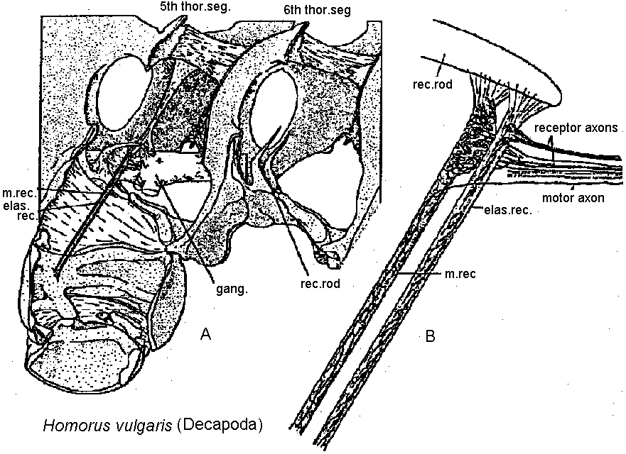 Homorus vulgaris (Decapoda). A. The muscular and elastic receptors in their normal position in the fifth thoracic segment; the receptor rods of the sixth segment are shown as they look when freed of connective tissue. B. Enlarged view of the same receptors. (Alexandrowicz & Whitear 1957). elos.rec., elastic receptors of the second leg; gong., ganglion of the ventral cord ; m. rec., muscular receptors of the second leg; rec. rod, receptor rod; thor. segm., thoracic segment.  Figure 25.10. Semidiagrammatic sketches of a myochordotonal organ: the propodite-dactylus organ of Carcinus maeflas, a crab. The organ itself consists .of a bunch of receptor nerve cells embedded in a strand of connective tissue which runs across the joint between the propodite and dactylopodite. C, small connective tissue attachment; e, apodeme of extensor muscle; f, apodeme of flexor muscle; h, hypodermis; n, nerve bundle to organ; N, main nerve bundle; a, elastic organ; P, attachment to small protuberance on the dactyl. (Burke 1954) Photoreceptor organ (光受容器官)Dermal photoreceptor (皮膚受容器)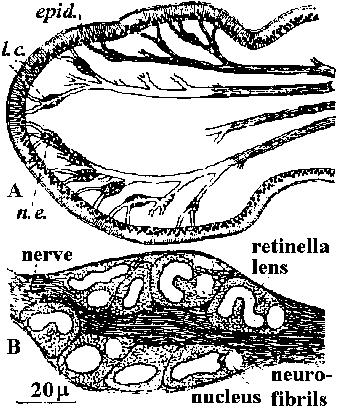 Fig. Photoreceptor nerve cells in the periphery. Lumbricus. A. Diagrammatic drawing of a sagittal section of the prostomium, showing the light cells both in the epidermis (epid.) and as enlargements along the coarse of nerves. l.c. light or photareceptar cell; n.e., enlargement on nerve due to cluster of light cells. B. One such swelling on a nerve, in longitudinal section. Reduced silver stain. (Hess. 1925)
inner limiting membrane (内境界膜/内境界板) 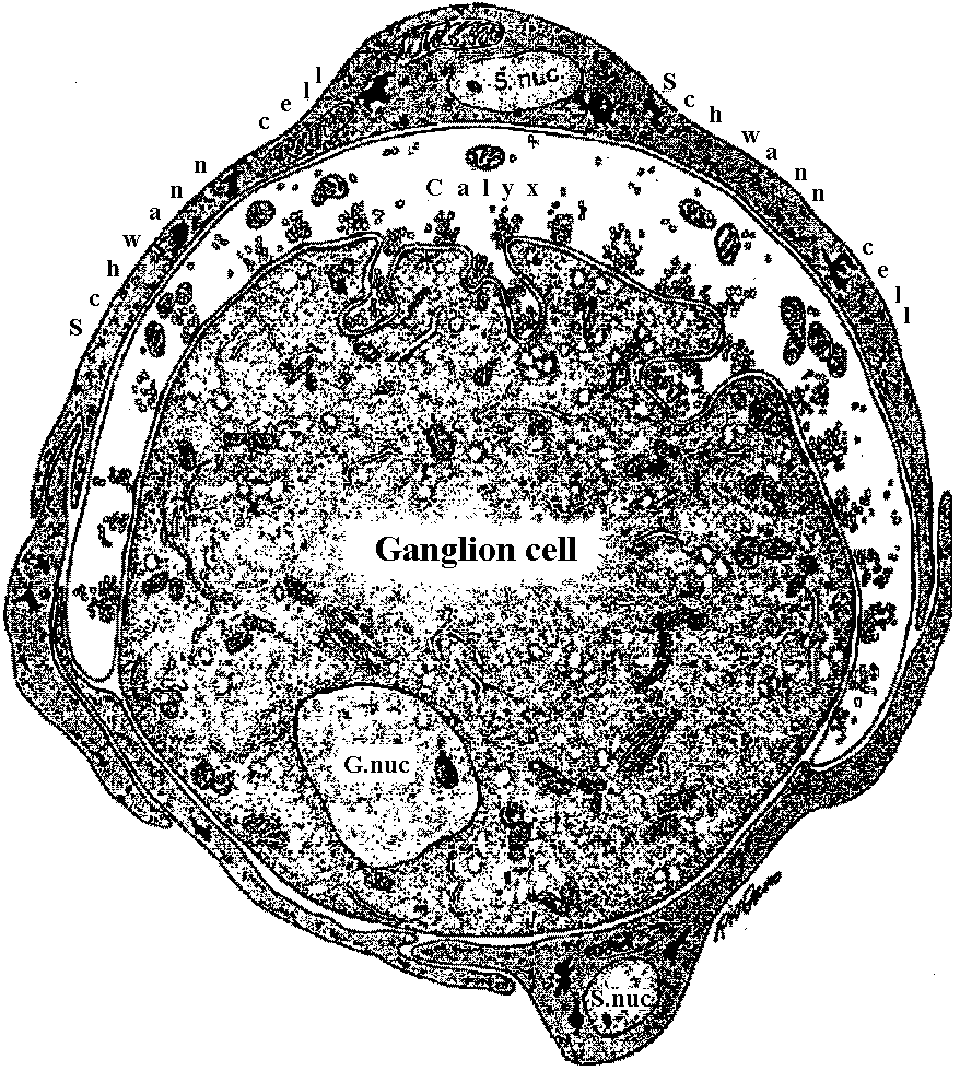 Figure 20-4. Diagrammatic representation of a cross section through a calyciform synapse in the ciliaiy ganglion of a chick. The presynaptic fiber has a cup-shaped ending (caltyx), which contacts a large area of the ganglion cell (axon not shown). The synaptic cleft is 300 to 400 Å units wide. Note the synaptic vesicles and mitochondria within the presynaptic ending. This is a synapse capable of both electrical and chemical synaptic transmission. G. nuc., nucleus of ganglion cell; S.nuc., nucleus of Schwann cell. (DeLorenzo 1960) 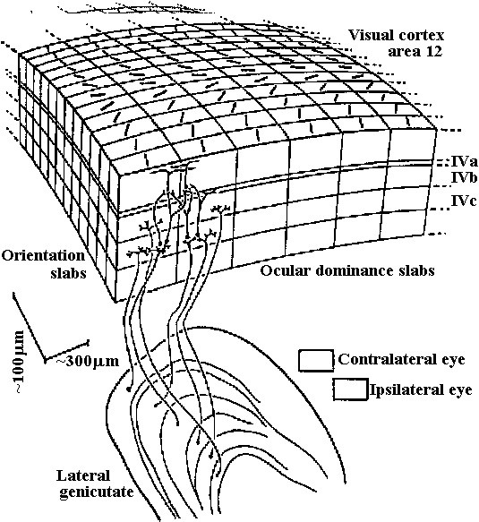 Fig. 3.12. Above. Postulated columnar organization of the primary visual cortex in the macaque. Below. Different layers of the lateral geniculate (adj. 膝の様に湾曲した) (i = ipsilateral, c = contrateral) send their output to adjacent parts of the cortex at the level of leayer IV. Here they innervate interneurons that distribute their influence both vertically up and down “ocular dominance columns” –really slabs– and laterally to adjacent columns, so that most cortical neurons can be driven binocularly, albeit with slightly stronger effect by the eye that provides primary input to that column. Perpendicular (垂直) to these wider (0.25 mm) columns are narrow (ca. 20-50 mm) “orientation columns” (actually slabs), and cells of which are selectively excited by signals having a certain orientation. Adjacent orientation columns differ by only a few degrees in their selectively. A family of these orientation columns would contain cells responsive to all possible orientations, all with essentially the same receptive field. Nearby would be cells organized into similar orientation and ocular dominance columns having a slightly displaced receptive field. The cellular circuity shown represents the input to an upper-level complex cell from two neighboring ocular-dominance columns, but from the same orientation column (Hubel & Wiesel 1972) Absorbtion spectra (吸収スペクトル)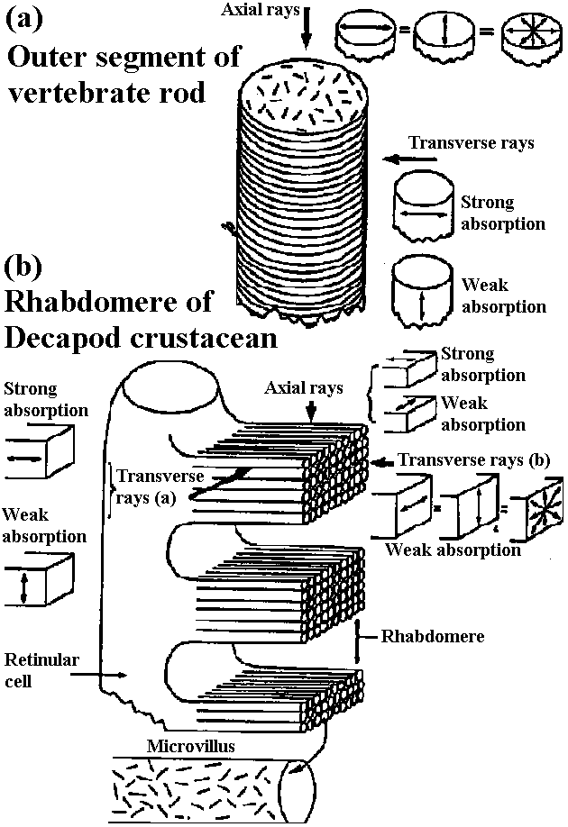 Figure 14-15. Orientation of visual pigment in the membranes of photoreceptors as revealed by dichroic absorption. A, In vertebrate rod and cone outer segments the chromophores lie randomly oriented in the planes of the disc membranes. Consequently, absorption of axially incident rays is independent of the plane of polarization. When illuminated from the side, however, the outer segments are dichroic: light polarized parallel to the planes of the discs (and thus the axes of many of the chromophores) is strongly absorbed, whereas light polarized at right angles to the discs is only weakly absorbed. B, The measurements of dichroism of decapod crustacean rhabdomeres are consistent with the view that the chromophores are randomly oriented in the planes of the photoreceptor membranes (i.e., in the tangent planes of the microvilli). Shown here is a single retinular cell and several of its tongues of microvilli. In an isolated rhabdom these tongues are interleaved with the rhabdomeres of other receptors (cf. Fig. 14.8C), but it is possible to irradiate a single band of microvilli with a laterally incident microheam. Absorption is isotropic when the beam is incident parallel to the microvillar axes, but it is dichroic when the light is incident at right angles to the microvillar axes. This latter condition is equivalent to axial illumination, as occurs in the living eye. Absorption is strongest when the light is polarized parallel to the microvillar axes. The measured dichroic ratio of 2 is consistent with random orientation as defined above; higher dichroic ratios might be expected if there were any orientation of the chromoohores oarallel to the microvillar axes.
|
Absorbtion spectra 吸収スペクトルTabel 14-2. The pigments of primate color vision. Figures in italics are from humans; others are from monkeys. Those designated “primate” are lumped data or are of unspecified origin. (p) = primate. Unit = lmax in nmBlue-sensitvie Green-sensitvie Yellow-sensitvie Technique of measurement cones cones cones 445, 455 535 570, 570 end-on microspcctrophotomctry 447 (p) 540 (p) 577 (p) end-on microspectrophotometry 450 525 555 end-on microspectrophotometry 440 (p) - - end-on microspectrophotometry - 535 (p) 575-580 (p) lateral microspectrophotometry 440 (?) 527, 535 565, 565 transmission spectrophotometry of retinal patches 430-440 530-540 565-595 fundal reflectometry 440 550 580-585 ┐ psychophysical measurements; 430 540 575 ┘ corrected for ocular and macular absorption 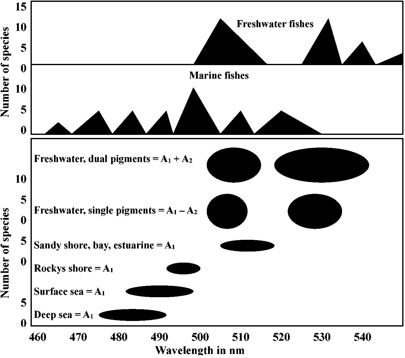 Figure 14-13. Distribution of visual pigments of teleost fishes. Each point represents the wavelength of maximal absorption of a pigment, obtained using partial bleaching analyses of extracts. The lower frame shows the data broken down by habitat. Data are from a number of sotirccs. (Crescitelli 1972) Auditory organ (聴覚器官)Phonoreception (distance sense) ⇒ evolved after terrestrial life = auditory nerve (聴神経)
Vertebrate: movement of medium (water current) 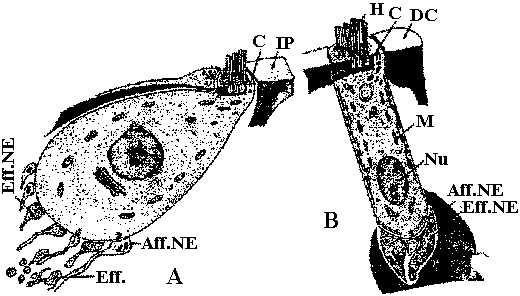 Fig. 27. Schematic drawing of an inner (A) hair cell and an outer (B) hair cell. C- centriole. Aff. NE- afferent nerve ending. Eff.NE- efferent nerve ending. IP- inner pillar. DC- deters cell. M- mitochondrion. Nu- nucleus.
Lateral line organ (canal, neuromast = fish): hair cell – directional sensitive
water flow 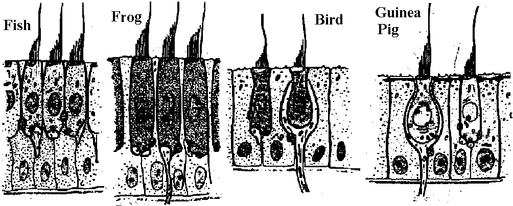 Fig. 4. Schematic drawing of the sensory cells in the vestibule epithelia in fish, frog, bird, and mammals, demonstratmg the shape of the oells sensory hairs and nerve endings. 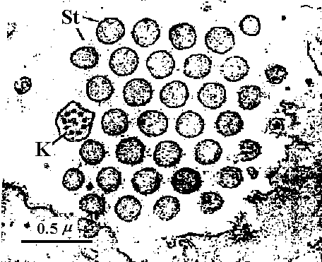 Fig. 5. Schematic drawing showing the ultrastructure of the stercocilium with its rootlet and the kinocilium and its basal body. The arrow indicates the direction of excitatory stimulation. 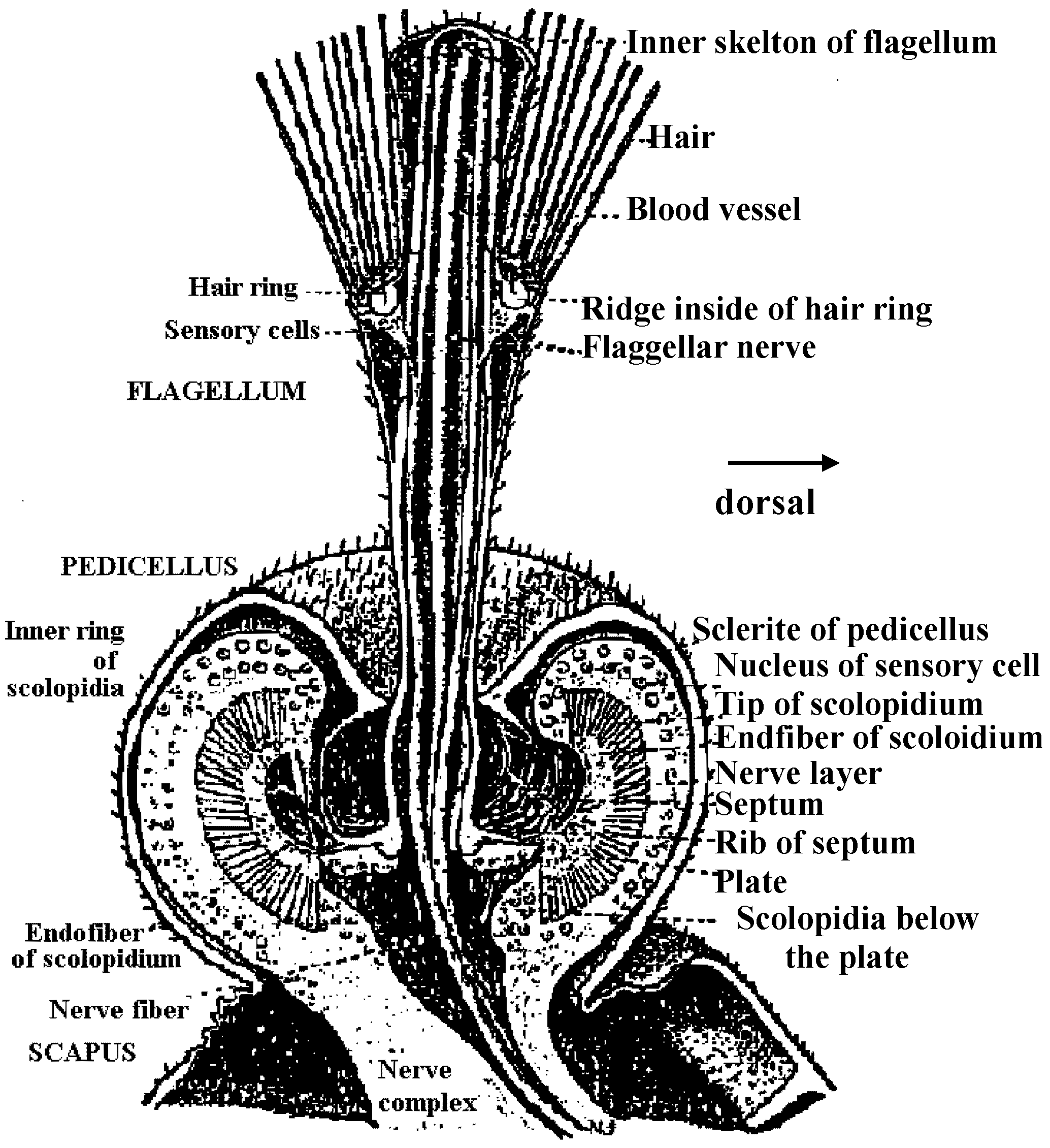 Fig. The organ of Johnston (mosquito) 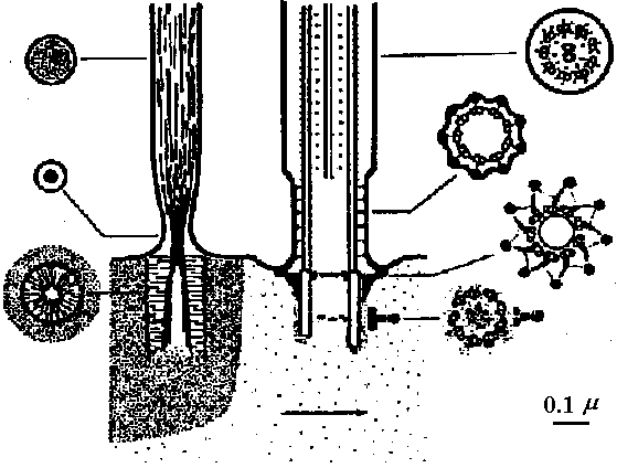 Fig. 6 Fig. 6
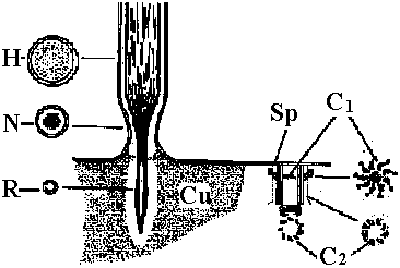 Fig. 31 Fig. 31Fig. 6. Cross section through a sensory hair bundle showing the regular arrangement of the stereocilia (SL) and the peripheral position of the kinocilium (K). Note the fibrillar network interwoven between the stereocilia. × 33,000. Fig. 31. Schematic drawing of structure of hairs and centriole on top of the hair cell in the organ of Corti. H- hair. N- neck of hair. R- rootlet. Cu- cuticle. C1-centriole 1. C2- centriole 2. Sp- spikes.  Fig 25.23. Schematic diagram of the structure of subgenual organs of insects: a, Orthoptera; b, Lepidoptera, and c, Hymenoptera. Part of the exoskelton of the bitia is removed to show the large trachea and the sensory neurons that are streached into it. The neurons respond with excitation to vibrations of frequencies from about 100 to about 10000. (Autrum et al. 1948) Olfactory (臭覚器)Static organ (平衡器)
|
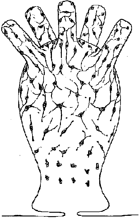
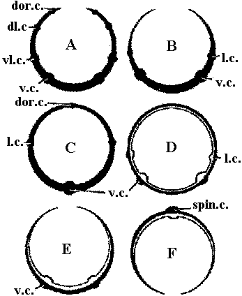
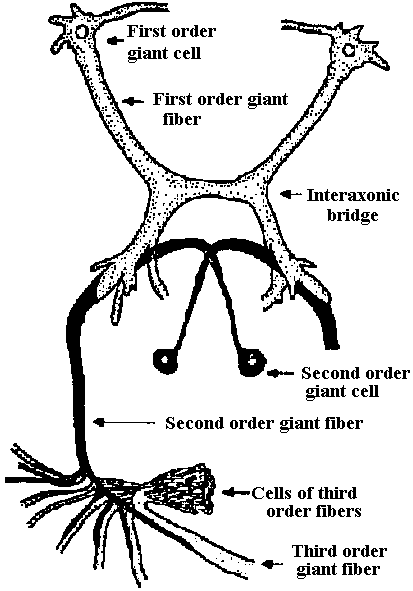
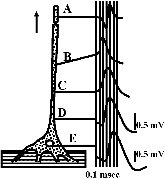 Fig. 2. The probable density of electrically excitable membrane compounds (dots) in different portions of the lobster stretch receptor (left) and the side of the spike trigger zone (right). The dots are sparse in the dendrite portion and become more dense along the axon, and particularly at the region of the trigger zone (Grampp 1966). The extracellular recording were of respnses to a stretch stimulus. The spikes occurred first at B, and propagated antidromically (C-E) to invade the cell body, as well as orthodromically (A) along the axon. Site B was about 0.5 mm from the cell body; site A was about 0.8 mm from B. Long vertical lines represent 100-μsec intervals. Short vertical lines represent 0.5 mV. A-D were recorded at the same amplification (Edwards & Ottoson 1958).
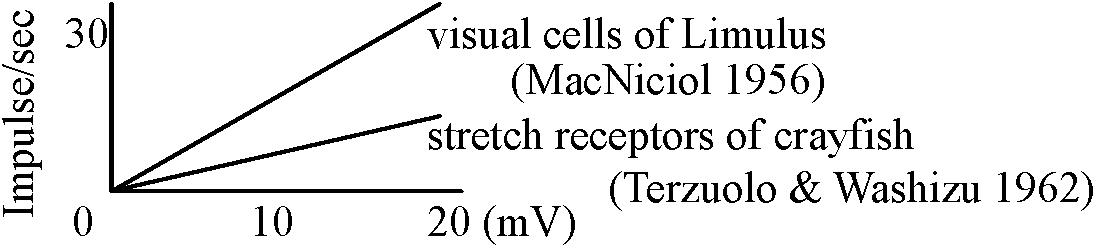
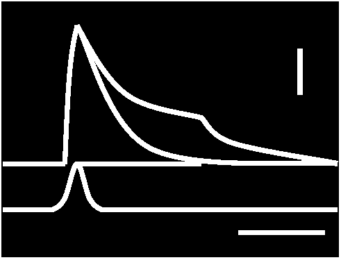 Responses of acceptor membranes: Fig. 17. Decay characteristics of receptor potential. Superimposed records of response to bried dynamic and maintained stretch to the same length. Time bar: 25 msec. Vertical bar: 0.5 mV (Ottoson & Shepherd 1970)
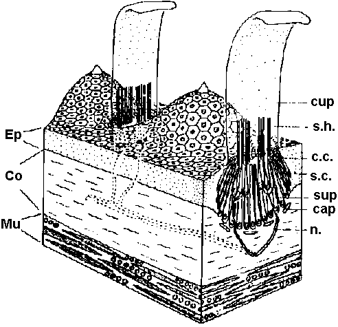
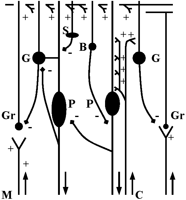
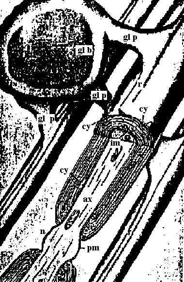
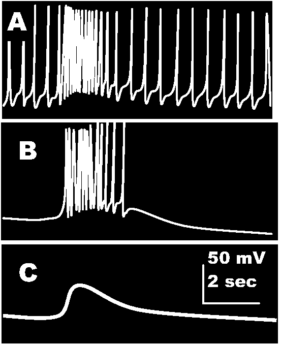
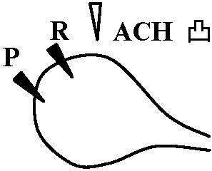 Fig. 20-32. Effects of brief (200 msec) electrophoretic application of aectyleholine (at arrows) on somatic membrane potential of a D cell of a ganglion of the opisthohranch (Gastropoda) Aplysia depilans. Above the records is a diagram of the set-up, showing the recording microelectrode (R), and the polarizing microeleetrode (P) inserted in the cell body and the acetyicholine-filled micropipet (ACh) applied to the outside of the cell. In A, the cell shows rhythmic activity, accelerated by ACh action. In B, the cell was slightly hyperpolarizcd to avoid spontaneous firing; ACh depolarizes transiently and induces spikes. In C, the cell was hyperpolarized further; the depolarizing wave produced by ACh action does not reach the firing level (Tauc & Gerschenfeld 1962)
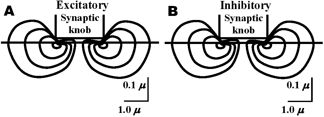
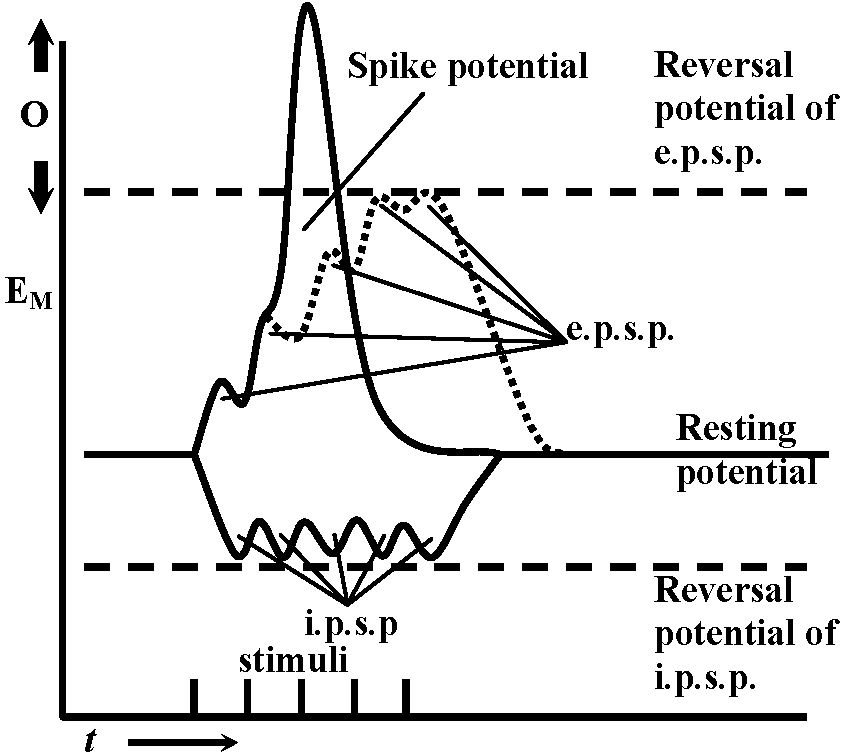
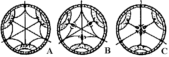
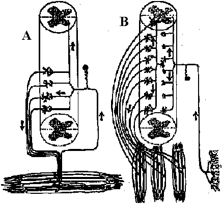
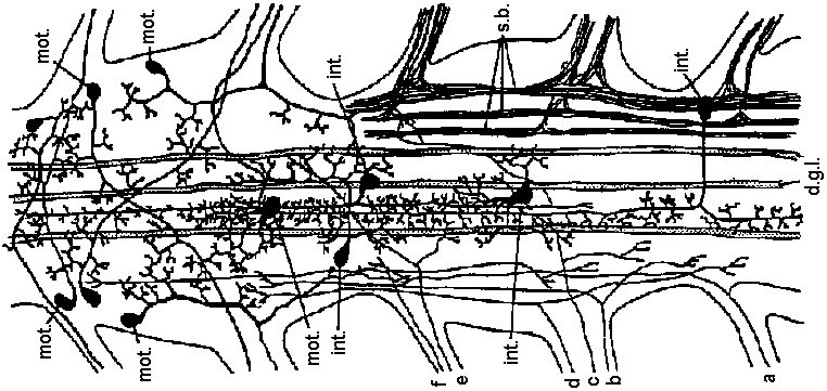
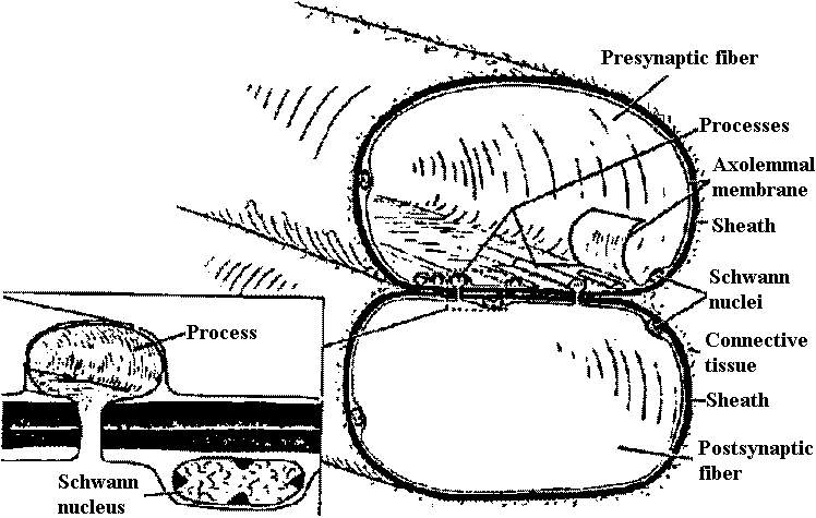
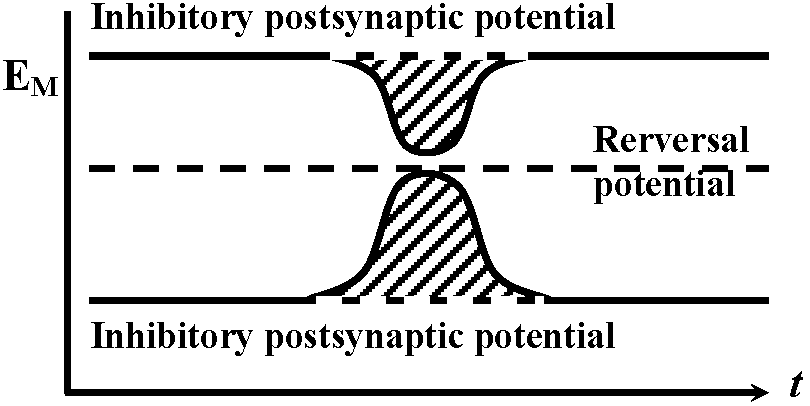
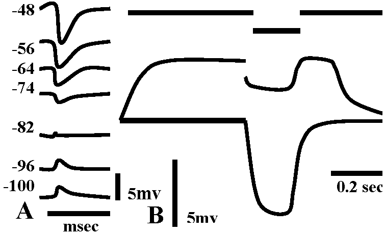
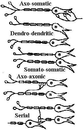
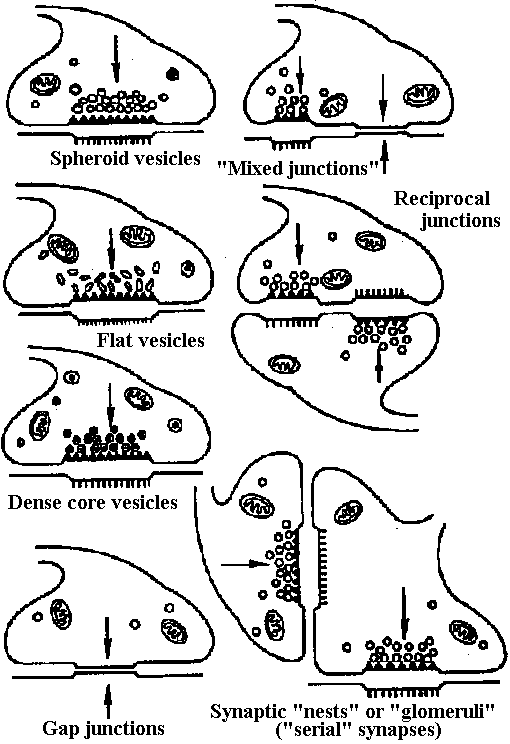
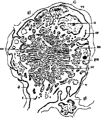
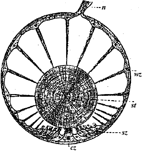 Fig. 25.19. Statocyst (平衡胞) of Mollusc, Pterotrachea (Heteropoda). The long cilia of the ciliated cells (wz) beat rhythmically, lifting the statolith (st) and allowing it to fall ou the hours of the sensory cells (sz). One of the latter is of particular size; it is called the central cell (cz). Depending on the position of the animal, different groups of sensory cells can be activated. The generated nerve impulses travel along the statocyst nerve (n) to the central ganglia (Stempel & Koch 1923)
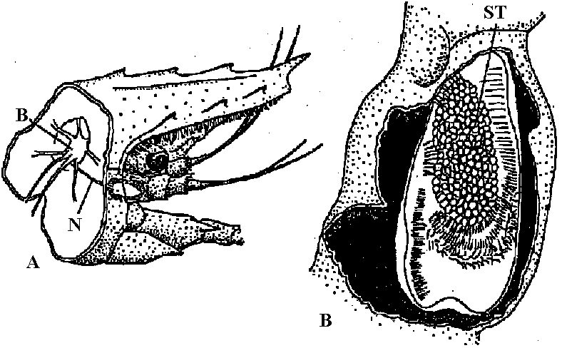
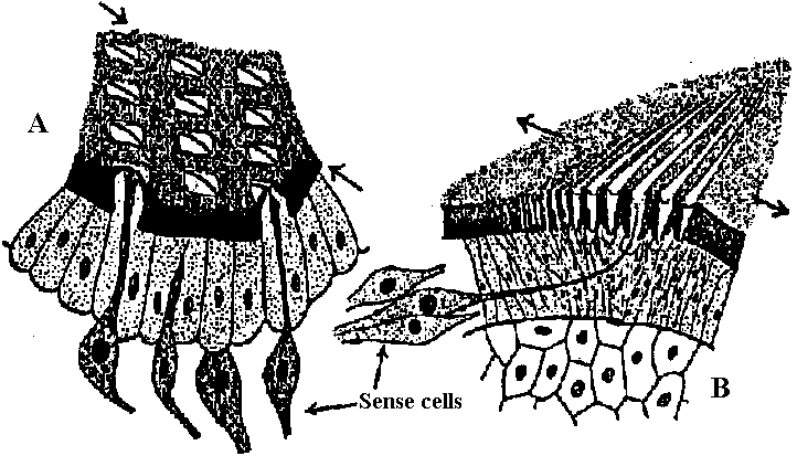
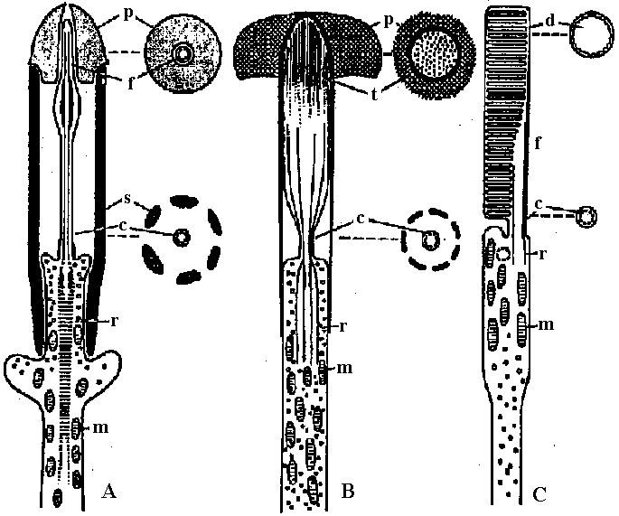
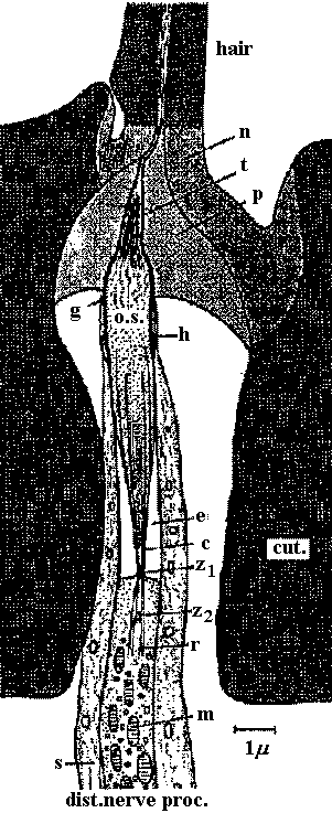 Fig. 2
 Fog. 5
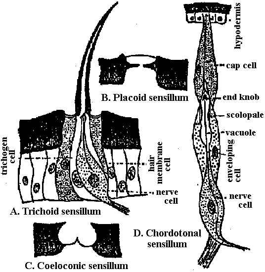
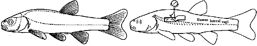
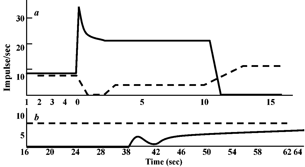
 Fig. 25.16. Movements of the cupulae of lateral line organs doe to water current ano wase pressure caused by an approaching object (a small disc). The diagram shows free sensory hillocks, canal organs, and canal pores. The direction of fluid movement is indicated by arrows. (Dijkgraaf et al. 1952)