(Upload on December 6 2025) [ 日本語 | English ]
Mount Usu / Sarobetsu post-mined peatland
From left: Crater basin in 1986 and 2006. Cottongrass / Daylily
HOME > Lecture catalog / Research summary > Glossary > Landscape
[satoyama, restoration ecology, geographic information system]
|
The main landscape is a combination of land systems in one geographical region (Naveh & Lieberman 1984) → successional landscape Three characteristics (Forman & Godron 1986)
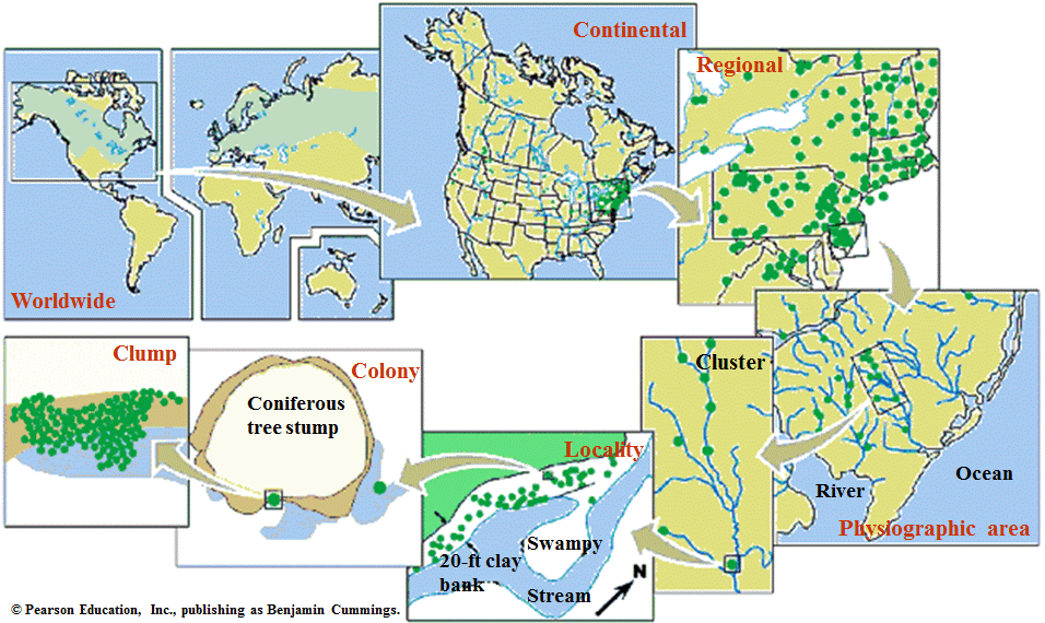
Scale-dependent factor (スケール依存性要因)Ecosystem at different spatial scales: We conceive the landscape as ecosystems, large and small, nested within one another in a hierarchy of spatial sizes (Row & Sheard 1981)

A hierarchy of scales for analyzing the geographic distribution of the moss Tetraphis The answer to the question "What limits geographic distribution?" may have different answers when analyzed at the continental scale versus the local scale of the individual tree stump. (Forman 1964) Level of landscapeTimeGeographical Species Centemporal Subspecies Seasonal Population Momental Individual Space Local Regional Provincial Continental* or insular |

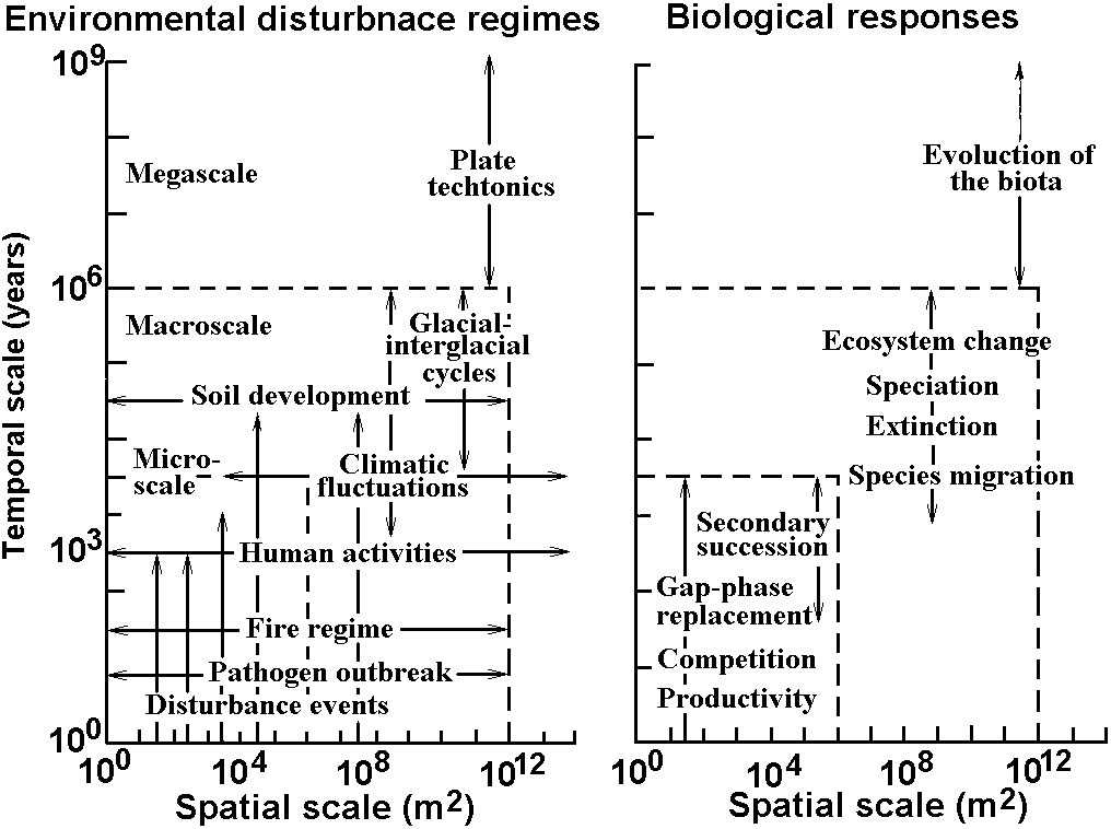
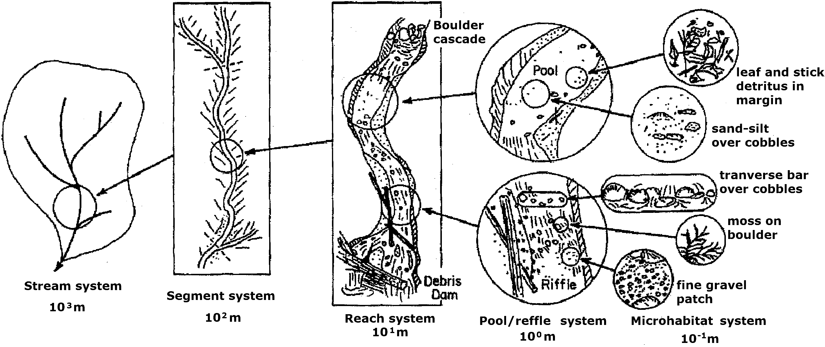
Fig. Relationship between spatial and temporal scales for various ecological phenomena. At the microscale, natural and human disturbances affect the establishment and succession of species. At the macroscale, regional climatic changes affect process such as species migration and displacement of ecosystems. At the megascale, plate techtonics, evolution of major groups, and development of global vegetation patterns are prominent. The five vertical arrows on the lower left represent disturbance events such as wildfire, wind damage, clear cutting, flood, and earthquake (Delcourt et al 1983).  Fig. 2. Hierarchical organization of a stream system and its habitat subsystems. Approximate linear spatial scale, appropriate to second-or third-order mountain stream, is indicated (Frissell et al. 1986) |
| Explanation | Suggested unit names | Approximate map-scale range | |
| I. | Large size landscape units (ca 10,000 ha or higher) | Bioclimatic region or zone, biogeoclimatic zone, life zone, vegetation zone, ecoregion, biome, ecological zone | National (small map scale) 1:1 million and smaller in map scale |
| II. | Intermediate size landscape units (ca 500 to 10,000 ha) | Land system, land form, forest cover type, plant formation, forest land type, forest ecosystem type | Regional-overview (medium map scale) 1:1 million to 1:100,000 (or occasionally up to 1:50,000) |
| III. | Small-sized landscape units (ca 1 to 500 ha) | Forest site type, forest habitat type, land type | Subregional or local-detailed (large map scale) 1:100,000 (or 1:50,000) up to 1:1,000) |
[ Naturalness ]
|
The study of land systems and of their relationship to one another, for each is set in the "environment" of its surrounding neighbors. In other words, landscape ecology is the science of landscapes, understood concretely as spatial and volumetric ecosystems in their regional contexts.
Landscape ecosystem approach: To take an ecosystem approach means that everyone attends to the conservation (保全) and sustainability of ecosystems, instead of sharply focusing on the productivity of individual or competing resources - which has been our traditional mode of operation. It means our focus is on landscape ecosystems rather than organisms which are parts of ecosystems. Landscape structure and function principles (Forman 1986)Landscapes are heterogeneous and differ structurally in the distribution of species, energy, and materials among the patches, corridors, and matrix present. Consequently, landscapes differ functionally in the flows of species, energy, and materials among these structural landscape elements.Biotic diversity principlesLandscape heterogeneity decreases the abundance of rare interior species, increases the abundance of edge species and animals requiring two or more landscape elements, and enhances the potential total species coexistence. |
Energy flow principlesThe flows of heat energy and biomass across boundaries separating the patches, corridors, and matrix of a landscape increase with increasing landscape heterogeneity.energy (エネルギー) · nutrients (栄養分) · species (種) → trophic level (栄養段階) Landscape change principleWhen undisturbed, horizontal landscape structure tends progressively toward homogeneity; moderate disturbance rapidly increases heterogeneity, and severe disturbance may increase or decrease heterogeneity.Landscape stability principleStability of the landscape mosaic may increase in three distinct ways, toward (a) physical system stability (characterized by the absence of biomass), (b) rapid recovery from disturbance (low biomass present), or (c) high resistance to disturbance (usually high biomass present). |
Closeness of heterogenous landsccapes supports the conservation of species, in particular, for species behave in large ranges
| Species | Landscape elements | Reference |
| Elk and deer | Forest, shrubland, and grassland-90% of use occurs within 200 m on both sides of forested edge | Thomas et al. 1979 |
| Ruffed grouse | Forest-equal proportions of four stand size classes, all intersecting at a common point to provide feeding (mature stand), breeding (pole stand), and roosting (regeneration stand) habitat | Gullion 1977 |
| Pheasant | Agricultural land-10 to 25% of land in hay crops that provide nesting and roosting cover | Joselyn et al. 1968; Warner 1981 |
| Canvasback, Redhead duck, Mallard duck, Canada goose | Agricultural land, grassland, and open water-agricultural residue and forage for feeding geese and mallards; fingernail clams and aquatic vegetation for feeding canvasbacks and redheads All species require terrestrial and aquatic habitats | Bellrose et al. 1979 |
| Black bear | Uplands and lowlands-acorns from upland oaks in summer and fall; acorns from lowland oaks in winter and spring | Landers et al. 1979 |
Evaluation of landscape heterogeneityExpanded from diversity index proposed by Shannon & Weaver (1949)
Region Streams/ Homes Dirt  Paved Woods Pastures Croplands
       reivers        roads roads
A        18       1    24     1     90     49        0
B        12       0    24     2     87     41        4
A χ² statistical test cannot be used to test the differences between these two sets of frequencies, because some are too small. Therefore, we compare the individual frequencies directly. For example, the contingency table for the presence or absence of streams and rivers in the 128 segments along each line is as follows:
    Region                        A     B     Total
    Streams and rivers present    18    12     30
    Streams and rivers absent    110   116    226
    Total                        128   128    256
|
The probability P of obtaining the results, when only 30 (that is, 12) of the 256 segments have streams or rivers, is
P = (30!226!128!128!)/(256!18!12!110!116!) = 0.079 The sum of this probability P and the probabilities of more extreme differences in streams and rivers between the two lines is 17%, well above the 5% statistical threshold. This means that these two lines do not differ significantly in the frequencies of streams and rivers present. We may therefore conclude that, based on streams and rivers only, the two lines are in the same landscape. The same calculation is made for each type of element. It then appears that the clearest difference between the two lines results from the croplands, for which the probability is only 6%. Thus, one can say that these two lines are in the same landscape, but that the croplands present in Nant 4 represent a significant difference between the two lines. |
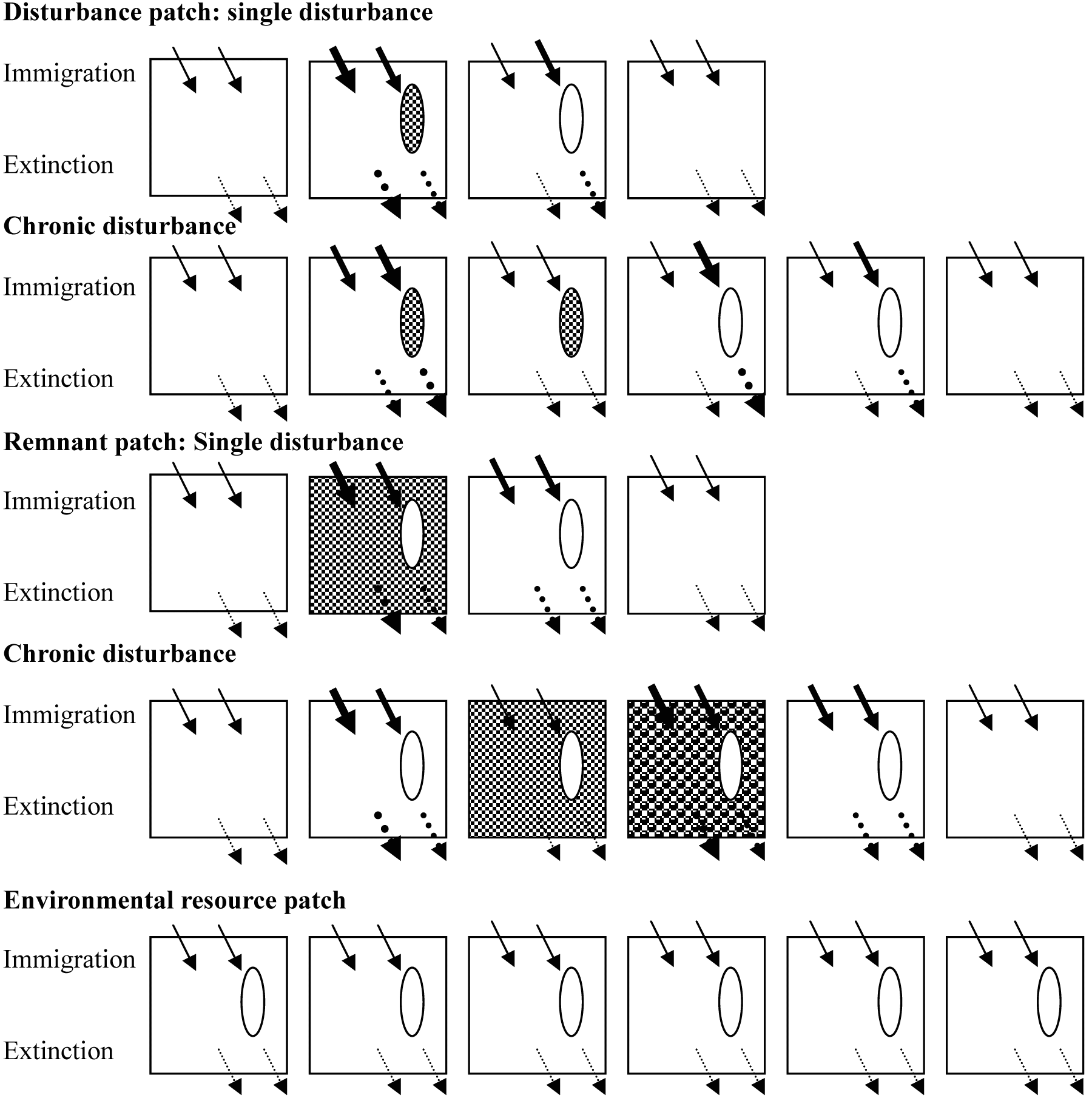
Patch structure of landscapePatches: size, distribution, shape, age, densityType: disturbance, remnant, and environmental resource patches + introduced patch (artificial)  Fig. Species immigration and extinction in patches of different origins. The square is an area of matrix containing a circle patch. Shading indicates an area being disturbed. The solid arrow is immigration and the dashed arrow is extinction. The thickness of an arrow is proportional to the estimated rate of immigration or extinction. Measures of patch characteristics in a matrixThe following measures proposed by different authors should be used with appropriate caution, since their dependability and generality in describing ecological patterns are as yet unclear.Shape of a patchDi = P/(P/2√Aπ), where Di is an index of the shape of patch i; P is the perimeter of the patch; and A is the area of the patch (Patton 1975; Game 1980; Bowen and Burgess 1981; Haggett et al. 1977).Isolation of a patchri = 1/n·Σn=1j=ndij, where rj is an index of the isolation of patch i; n is the number of neighboring patches considered; Σ is the sum of; and dij is the distance between patch i and any neighboring patch j (King 1969; Bowen & Burgess 1981). |
Accessibility of a patchai = Σn=1j=ndij, where ai is an index of the accessibility of patch i; dij is the distance along a linkage (e.g., a forest corridor or hedgerow) between patch i and any of the n neighboring patches j (Lowe & Moryadas 1975; Bowen & Burgess 1981).Interaction among patchesIj = Σn=1j=n(Aj/dj2), where Ij is the degree of interaction of patch i with n neighboring patches; A is the area of any neighboring patch j; and d, is the distance between the edges of patch i and any patch j (Whitcomb et al. 1981; MacClintock et al. 1977).Isolation of patchesD = Σ(σx2 + σy2), where D is an index of the isolation of all patches present. Patches are located on a grid with x and y coordinates. The average location and the variance for all patches are calculated for the y coordinate. σx2 and σy2 are the variances on the x and y coordinates, respectively. This equation is based on the "standard distance index" (Lowe & Moryadas 1975; Bowen & Burgess 1981).Dispersion of patchesRc = 2dc(λ/π), where Rc is an index of dispersion; dc is the average distance from a patch (its center or centroid) to its nearest neighboring patch; and λ is the average density of patches. Here Rc = 1 with randomly distributed patches; Rc < 1 for aggregated patches; and Rc > 1 (up to a maximum of 2.149) for regularly distributed patches. This equation is a measure of aggregation (Clark & Evans 1954, 1979; Pielou 1977).Barriers and edgeAny distinctive habitat not "ISLANDY", e.g., water (sea, fresh), deserts, landUrban lots → grasses/compositae Oceanic islands → orchids, lower plants ↓ Distance Barriers are not domestic: dispersal (wind, animal, self, gravity etc.), disharmony
Colonization = ∫(distance + island size + barrier)dt Extinction = chance / lower habitat complexity / lack of refuge / competition / succession / lack of rescue Equilibrium: colonization = extinctionbreaching barriers / disharmony Relaxation: persistence and stability |
Patternization (or patterning of classification)For the recognition of landscape patterns, we classify landscapes based on similarities or dissimilarities.Region
natural region (自然地域): topography, climate, population density = landscape |
Transition matrix (トランジッションマトリックス)Spatio-temporal change → diversity, abundance, age distribution, size distribution, etc. → expressed by matrix modelLeslie matrix
______________________Pastures in the__Cultivated fields in (87.5% × 1000 ha) + (50% × 1000 ha) = 875 + 500 = 1375 ha and the area of cultivated fields will be (12.5% × 1000 ha) + (50% × 1000 ha) = 125 + 500 = 625 ha At the end of the second year, the areas are
(87.5% × 1375) + (50% × 625) = 1516 ha in pasture, and After the third year, the areas are
(87.5% × 1516) + (50% × 484) = 1568 ha in pasture, and Continuing these calculations for several years gives the following:
1568 - 1588 - 1596 - 1598 - 1599 - 1600 - 1600 ha in pasture |
|
|
Def. Original vegetation (原植生): vegetation developing without human impact ⇔ Def. Secondary vegetation (代償植生): vegetation develped under human impact Def. Potential natural vegetation (潜在自然植生), PNV vegetation that is expected given environmental constraints (climate, geomorphology, geology) without human impact Satoyamasemi-natural environments comprised of human activities and diverse ecosystems such as (secondary) forests, wetlands including rivers, farmlands, and grasslands, in particular, distributed in East Asia (Takeuchi et al. 2003)
|
Unit ecosystemTo protect biodiversity, link between ecosystems is important. Due to urbanization and/or farm retirement, the area of Satoyama is decreasing. |
|
Def. Landscape architecture is the art of arranging land so as to adapt it most conveniently, economically and gracefully to any of the varied wants of civilization (Cleveland HWS, 1973) Landscape architecture (総合景観) =
Landscape architecture (建築景観) + Hibiya Park (日比谷公園)1989(M22) decided the construction (designed based on German parks by Honda)1902 groundbreaking - 1903 grand opening Mt. Mikasa (三笠山)The area west of the tennis courts including this hillock is called Mt. Mikasa. The hillock is an artificial oen, made with leftover soil from the construction works making ponds when the park was constructed. At the time it was created, the physical shape of the whole area resembled three woven hats, or kasa in Japanese, so that it got its name "Mikasa", meaning three woven hats. Due to improvement works such as the construction of tennis courts, the mountain shape has changed, still the name of it remains as the original name.The place of death of Date Masamune, the founder of the Sendai Clan (仙台藩祖 伊達政宗 終焉の地)This is where the Sendai Clan's main Edo (Tokyo) residence, Sotosakurada Kamiyashiki, was located from the period of the founder, Date Masamune, to the third Lord, Date Tsunamune. In Keicho 6 (1601), Masamune was given a residence in Edo by the Shogun, Tokugawa Ieyasu. This residence in Sotosakurada was used as his main residence in Edo until Kanbun 1 (1661). The grounds of the residence spanned from the western shore of Sinji Pond to eastern tip of the tennis courts, and from the road alongside Hibiya-bori Moat in the north to the area around the Small Open-Air Consert Hall in the south. The records state that, at this residence, Masamune hosted Tokugawa Ieyasu on three occasions, in addition to both 2nd Shogun Hidetada and 3rd Shogun Iemitsu on four occasions each. Masamune's life ended here in May, Kan'ei 13 (1636) at 70 years of age during his stay in Edo under the system of altering residence. |

Stone basin (石枡)The water tank curved out of stone in an Edo period water supply facility which was connected to the wooden pipe aqueduct. There are some of the same remaining throughout the park. A giant stone bollowed out into a square shape, it has a grand design. Some of them have their location inscribed insde them. These basins were installed in various places along the main road of Edo City, from which water was supplied to the residences of feudal lords.Jindai Botanical Gardens (神代植物公園)History of the Name of the Jindai Botanical Gardens During the Eco period (1600-1868), the area around the Jindaiji temple was known as Jindaiji-mura (village of Jindaiji). In 1889 and administrative reorganization combined the municipalities surrounding the temple, including the villages of Sazu and Murasaki, to create the new village of Jindai. That new Jindai name means “the age of gods” and has the same pronunciation but a different meaning than the name of the temple. In 1940 the government of Tokyo designated this site as an attack shelter zone and the name was changed to Jindai Greenspace. The government purchased about 710,000 m2 of land and began using it for nurseries and gardens. As a result of agricultural reform after the end of Second World War, about three quarters of the land was conveyed to farmers. In 1961, the government created this garden on about 250,000 m2 of land, comprising the remaining public land and repurchased land, and carried on the former name of the greenspace with the name Jindai Botanical Garden. In 1955 the village of Jindai became part of the city of Chofu which is the present location of the Jindai Botanical Garden. |
(Glasson 1974)
|
National land studies or territorial studies (国土学): (unique to Japan) omprehensive understanding of national land utilization, conservation, development, and management → research on methods for sustainable development
= geography + geology + environmental science + economics + political science, etc. Regionalism (Odum WH)regionalism as scienceregionalism as frontier のregionalism as governmental avenue or technique regionalism as motive or objective rural community + urban community = social community Britain1989 "Tomorrow: A peaceful path to the reform"
Howard's garden city (e.g., Letchworth, Welwyn)
= self-contained + balanced community Social city: central city for community of garden cities present metropolis development: public housing corporation → public welfare, construction, agricultural community, trade-industry 1945 Distribution of industrial act1946 New towns act 1947 Town and country planning act the foundation of modern town and country planning in UK 1990 Town and country planning act for England and Wales1997 Town and country planning (Scotland) act 2004 Planning and compulsory purchase act 2008 Planning act 2011 Localism act Netherlands (Polder planning)Total planning:
early polder planning Amsterdam, Noord Holland, Zuid Holland Zwiderzee polder
|
mid-and long-term planning: planed based on the potential future floods → lead by numerical economics
Criteria to conduct land reclamation (in general): benefit/cost > 1 → do reclamation → introduced to Japan (Hachiro-gata) = case of failure
2.5 ha (4700 houses) → 10 ha (910 houses) → [acreage reduction] → 15 ha (7.5 ha rice field, 7.5 ha crop field) The former West GermanySocial and economic structure of West Germany(economic association / labor association) + regionality Local system of West Germany
Center_______Commonwealth Tennessee Valley (テネシー峡谷)1933 Tennessee Valley Authority (テネシー峡谷開発公社, TVA)The first regional development plan worldwide 1962: Ronald Reagan fired by General Electric for criticizing TVA
Major ideas (controversial) Regional landscape planning (地域景観計画)local planning + local planning + local planning ≠ regional planning - changes in dimensions |
| Practice (実践) | |
|---|---|
|
Def. Yard tree or garden tree (庭木): a tree planted in a yard or garden, primarily for ornamental, practical or landscape purposes
Ornamental: aesthetic appeal, seasonal flowers, foliage |
The species and forms of garden trees used depend on how they are appreciated, the purposes and functions they serve, and the style of gardening |
Joint public-private venture (第三セクター)= joint public-private venture or quasi-public corporation (company or enterprise), in JPN usage
≈ public–private partnership (PPP) |
Third sectorin US usage = not-for-profit industry
nonprofits |