(Upload on August 29 2025) [ 日本語 | English ]
Mount Usu / Sarobetsu post-mined peatland
From left: Crater basin in 1986 and 2006. Cottongrass / Daylily
HOME > Lecture catalog / Research summary > Glossary > Mathematics > Statistics
|
Too many people use statistics as a drunken man uses a lamppost, for support but not for illumination. (Finney 1997) Raw data, ≈ primary data (生データ)data collected from a sourcethe data have not been subject to any manipulation, such as outlier removals, corrections and calibrations
raw data are the evidnece to deomonstrate the correct information → McNamara, Robert Strange (1916-2009), US government official the logical error of excessively relying on quantitative data to make decisions while ignoring important qualitative factors that are hard to measure Ex. Body counts in Vietnam War as a measure of successthis approach ignored critical qualitative factors:
guerrilla warfare - difficulties in body counts |
Statistical ecology (統計生態学)= ecological statistics (生態統計学)referring to the application of statistical methods to the description and monitoring of ecological phenomena ≈ overlapping mostly with quantitative ecology (定量生態学, s.l.) adding momentum for quantification after 1960's - transcending descriptive ecology (記載生態学) Ex. 1969 International Symposium on Statistical Ecology (New Haven, Conn.) |
[ statistical test | determinant ]
|
Def. Trial (試行)
Experiment: conducting a trial or experiment to obtain some statistical information Def. Event (事象): a set of outcomes of an experiment (a subset of the sample space) to which a probability is assignedExpression: A, B, C, … Def. Complementary event (余事象): AC, BC, CC, …Combination and permutation (組み合わせと順列)Combination (組み合わせ)Def. A selection of items from a collection, such that (unlike permutations) the order of selection does not matterEx. "My fruit salad is a combination of apples, grapes and bananas." → combination nCr =nC0 = nCn = n!/n! = 1 Eq. nCk = n!/{k!(n – k)!} = n!/[(n – k)!{(n – (n – k)}!] = nCn–k Th. nCk + nCk+1 = n+1Ck+1 Pr. nCk + nCk+1 = n!/{k!(n – k)!} + n!/[(k + 1)!{(n – (k + 1)!}]
= n!/{k!(n – k – 1)!}·{1/(n – k) + 1/(k + 1)} |
Th. (1) knCk = nn-1Ck-1, (2) n-1Ck + n-1Ck-1 = nCk Pr. (1) knCk = k·(n!/(k!(n - k)!) = (n·(n - 1)!)/((k - 1)!(n - k)!) = n·((n - 1)!)/((n - 1) - (k - 1))! = nn-1Ck-1 ___(2) n-1Ck + n-1Ck-1 = ((n - 1)!)/(k!(n - 1 - k)!) + (n - 1)!)/((k - 1)!(n - k)!)
= ((n - k)·(n - 1)!)/(k!(n - k)!) + (k·(n - 1)!)/(k!(n - k)!) Permutation (順列)= an ordered combinationDef. The act of arranging the members of a set into a sequence or order, or, if the set is already ordered, rearranging (reordering) its elements - a process called permuting
Scales and attributes
|
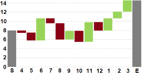
GraphHistograms (ヒストグラム)Bar graph (棒グラフ): bars with heights or lengths proportional to the values that they represent
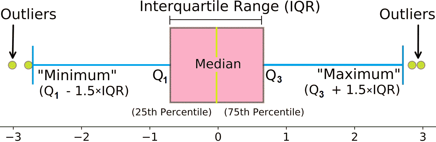
Vertical bar graph (column chart) Box-and-whisker plot (箱髭図): a standardized way of displaying the distribution of data based on a five number summary
4. "maximum": Q3 + 1.5×IQR Pie chart (円グラフ) Multi-pie chart Multi-level pie chart Sunburst chart (サンバーストチャート) Radar chart (レーダーチャート) |
Contour plot (等高線図) Spherical contour graph Venn diagram (ベン図) Spider chart (クモの巣グラフ) Mosaic or mekko chart Line graph (線グラフ) Multi-line graph Scatter-line combo Control chart (管理図) 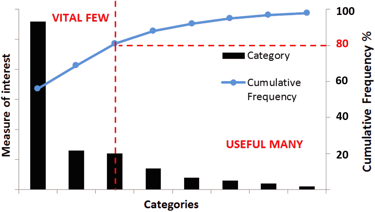
a bar chart ranking categories by frequency or impact = scatterplot, scatter graph, scatter chart, scattergram and scatter diagram
using Cartesian coordinates to display values for typically two variables for a set of data Stacked area chart Trellis plot (Trellis chart and Trellis graph) Trellis line graph Trellis bar graph Function plot Binary decision diagram (BDD, cluster, 二分決定グラフ) Hierarchy diagram (階層図) Circuit diagram (回路図) Flowchart (フローチャート, 流れ図): a type of diagram that represents a workflow or process ⇒ Ex. TWINSPAN Pictograph (統計図表): using pictures instead of numbers3D graph |
Mean vs average: Mean, median and mode are types of averagesArithmetic mean (算術平均), m or x-= (x1 + x2 + x3 + … + xn)/n = 1/n·Σk=1nxk
affected by the outlier(s). may loose the representativeness when the data are censored Geometric mean (幾何平均, xg)= (x1·x2 … xn)1/n∴ logxg = 1/n·(logx1 + logx2 + … + logxn) = 1/n·Σk=1nlogxk (∀xi > 0) used for change rate Harmonic mean (調和平均), mhDef. Mean square (2乗平均), MS(x) = 1/nΣi=1nxi2Eq. σ2 = (MS(x))2 - m2 (m: mean. σ2: variance) Pr. σ2 = 1/nΣi=1n(xi - m)2 = 1/nΣi=1nxi2 - 1/nΣi=1n2mxi + 1/nΣi=1nm2 ∴ σ2 = MS(x)2 - 1/nΣi=1n2mxi + 1/nΣi=1nm2 - 1/nΣi=1n2mxi = - 2m·1/nΣi=1nxi = -2m2
∴ σ2 = m2 - 2m2 + 1/nΣi=1n2m2, here, Σi=1n1 = n Circular statistics (角度統計学)≈ directional statistics and spherical statistics
GraphHistogramCircular raw data plot (円周プロット) (Nightingale) rose diagram (coxcomb chart, kite diagram, circular graph, polar area diagram 鶏頭図) Each category or interval in the data is divided into equal segments on the radial chart. Each ring from the center is used as a scale to plot the segment size |
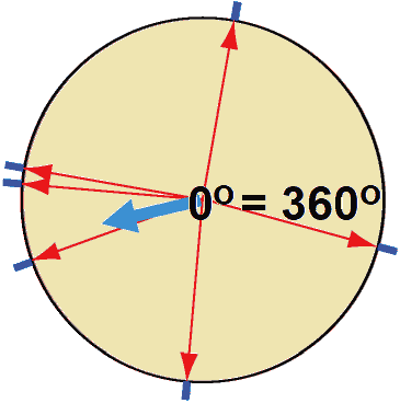 Q. Mean of 1° and 359°
A. Correct: 0°, incorrect: (1 + 359)/2 = 180° Q. Obtain mean of (80°, 170°, 175°, 200°, 265°, 345°) A. × (80° + 170° + 175° + 200° + 265° + 345°)/6 = 206° Def. mean (Θ) of vectors, (RcosΘ, RsinΘ)
= 1/N(Σicosθi, Σisinθi),__R: angle. θ: length 
Θ = 191° Def. (circular) variance (円周分散), V ≡ 1 - R (0 ≤ V ≤ 1)Def. (circular) standard deviation (円周標準偏差), S ≡ √(-2·logR)__(0 ≤ S ≤ ∞) Def. mean angular deviation, v ≈ S = √(2V) when V is sufficiently small = √{2(1 - R)} Circular uniform distribution (円周一様分布)
p.d.f. f(θ) = 1/(2π)__(0 ≤ θ ≤ 2π) P(θ) = exp(κcos(θ - μ)/(2πI0(κ)) ∝ exp(κcos(θ - μ)) parameters = (μ, κ), μ = mean, R = Ii(κ)/I0(κ) called normal distribution on the circumference of circle Statistical tests of circular dataWhen von Mises distribution is assumed, the test is parametricRayleigh test (Rayleigh z test) a test for periodicity in irregularly sampled data Kuiper test, H0: ƒ(θ) ~ P(θ)a test if the sample distribution follows von Mises distribution Mardia-Watson-Wheeler test, H0: Θ1 = Θ2a test if the two samples are extracted from the same population |
|
Def. statistical phenomenon (統計的現象) = probabilistic event/stochastic event (確率的現象): satisfied the two conditions shown below
1) non-deterministic (非決定論的) |
Poisson distributionLaw. Law of small numbers (ポアソンの小数の法則)Bi(n, p), np = λ (= constant), n → ∞, p → 0 ⇒ lim(nCk)pkqn–k = e-λ·(λk/k!) Pr. np = λ = constant P(X = k) = nCkpkqn-k
= [{n(n – 1) … (n – k + 1)}/k!]·(λCn)k·(1 – λ/n)n–k
-λ/n = x → (n → ∞ → x → 0) |
Th. Reproducing property of Poission distribution (ポアソン分布の再生性)
X1⫫X2, X1~P(λ1), X2~P(λ2) ⇒ Y = (X1 + X2)~P(λ = λ1 + λ2) Pr. P(X + Y = n) = Σk=0nP(X = n - k)P(k)
= Σk=0ne-λ1·λ1n-k/(n - k)!·e-λ2·(λ1k/k!) |
|
Def. Mean (expectation, 平均/期待値)
E(X) = mx = 1/nΣi=1nxifi = Σn=1hxiX(fi/n)
cp. s2 = 1/nΣi=1n(xi – mx)2 [√V(X): standard deviation] 1. E(aX + b) = aE(X) + b 2. E(X1 + X2 + … +Xn) = E(X1) + E(X2) + … + E(Xn) 3. XΠY → E(X·Y) = E(X)·E(Y) Pr. (Case, discrete) 1. E(aX + b) = Σk(axk + b)P{X = xk} = aΣkxkP{X = xk} + bΣkP{X = xk} = aE(X) + b |
2. E(X + Y) = Σk(xkP(X = xk) + ykP(Y = yk))
= ΣkxkP(X = xk) + ΣkykP(Y = yk) = E(X) + E(Y) → extension 3. E(X·Y) = Σk(xkP(X = xk)·ykP(Y = yk)= Σk(xkP(X = xk)·ΣkykP(Y = yk) = E(X)E(Y) [条件より] Th. Characteristics of variance (分散の性質)1. V(aX + b) = a2V(X) Ex. V(X + b) = V(X), V(2X) = 4V(X) 2. V(X) = E(X2) – E2(X) 3. V(X1 + X2 + … + Xn) = V(X1) + V(X2) + … + V(Xn) + 2Σi<j(Xi, Yj) 4. XΠY → V(X1 + X2 + … + Xn) = V(X1) + V(X2) + … + V(Xn) Pr. 1. V(aX + b) = E{aX + b - E(aX + b)}2 = E{a(X - E(X))}2 = a2V(X) 2. V(X) = E{X2 - 2E(X)X + E2(X)} = E(X2) – 2E(X)E(X) + E2(X)
= E(X2) – E2(X) = E2{(X1 - E(X1)) + (X2 - E(X2)) + … + (Xn - E(Xn))} // 4. (demonstrate cov(Xi, Xj) = 0) |
|
Th. 0. Chebyshev's inequality (チェビシェフの不等式) = Bienaymé–Chebyshev inequality For any probability distributions, no more than 1/λ2 of the distribution values can be λ or more standard deviations (SDs) away from the mean (or equivalently, over 1 − 1/λ2 of the distribution values are less than λ SDs away from the mean) Form 1) Σ|xi–x|≥λs ≤ n/λ2, or Σ|xi–x| < λs ≥ n(1 – n/λ2) Pr. ns2 = Σi=1n(xi – m)2 = Σ|xi – mx| ≥ λs(xi – m)2 + Σ|xi – mx| < λs(xi – m)2
≥ Σ|xi – x| ≥ λs(xi – m)2 Pr. λ = ε/√V(X) ∴ ε = λ√V(X) Th. Chebyshev's theorem チェビシェフの定理 {Xn}, XiΠXj (i ≠ j), V(Xk) ≤ c (c = constant, k = 1, 2, … , n), ∃ε > 0 → lim{|1/n·Σk=1nXk – 1/n·Σk=1nE(Xk)| < ε} = 1 |
Pr. V(1/n·Σk=1nXk) = 1/n2·1/n·Σk=1nV(Xk) ≥ c/n
Chebyshev's inequality → ≥ 1 – 1/ε2·V(1/nΣk=1nXk) ≥ 1 – c/nε2
limP(|1/nΣk=1nXk – 1/nΣk=1nE(Xk)| < ε) ≥ 1, P ≤ 1 X1, X2, … Xn: independence, E(xi) = μ, V(xi) = σ2
→ lim{|(X1 + X2 + … + Xn)/n – μ| ≥ ε} = 0
= 1/n·{E(X1) + E(X2) + … + E(Xn)} = 1/n·nμ V(m) = V((X1 + X2 + … + Xn)/n) = 1/n2·E(X1 + X2 + … + Xn)/n) = 1/n2·{(E(X1) + E(X2) + … + E(Xn)) = 1/n2·nσ2 = σ2/n
P{|(X1 + X2 + … + Xn)/n - μ| > λ·σ/√n} ≤ 1/λ2, λ·σ/√n ≡ ε, λ = √(n)/σ·ε |
|
____________ ↗ Sample (x1, x2, … xn) ____________ ↗ Sample (x'1, x'2, … x'n) [ population ] → Sample (x''1, x''2, … x''n) _____└─────────┘ Statistical theory Def. population (母集団): the total set of observations that can be made Ex. the set of GPAs of all the students at Harvard Def. sample (標本): a set of individuals collected from a population by a defined procedure |
Census and samplingCensus = complete census or survey (全数調査)Ex. national population census (国勢調査) Sampling survey = sample inquiry, sampling investigation (標本調査) |
The most popular and the central model is the normal sample theory in mathematical statisticsOutlier (外れ値)= abnormal, discordant or unusual value (異常値)Def. a data point that differs significantly from other observations affecting greatly the mean ⇔ affecting leass or none the median and mode |
Detection of outliersFirstly, need to construct the assumption of distribution (that is usually normal distribution)Tietjen-Moore Test (Tietjen-Moore 1972): detecting multiple outliers in a univariate data set that follows a normal distribution
= a generalized or extended Grubbs' test Standardization (標準化)(Zar 1996) Data transformation (データ変換) |
Regression analysis (回帰分析)Def. correlation coefficient (相関係数), r= (Pearson) product-moment correlation coefficient (積率相関係数) TerminologyMatrix (行列)Correlation matrix (相関行列): a table showing correlation coefficients between variablesPositive definite (正値/定符号): displaying the coefficients of a positive definite quadratic form Covariate (共変量): a statistical variable that changes in a predictable way and can be used to predict the outcome of a study |
Covariance matrix (共分散行列) = auto-covariance matrix, dispersion matrix, variance matrix or variance–covariance matrix (分散共分散行列) a square matrix giving the covariance between each pair of elements of a given random vector Unbiased estimator (不偏推定量): an estimator of a given parameter is said to be unbiased if its expected value is equal to the true value of the parameter - an estimator is unbiased if it produces parameter estimates that are on average correct Variance inflation factor, VIF (分散インフレ係数): the quotient of the variance in a model with multiple terms by the variance of a model with one term alone |
|
Correlation (相関): f(x, y) → y
x: independent variable, explanatory variable, or predictor The function relates the expected value of the response to the linear predictors in the model. A link function transforms the probabilities of the levels of a categorical response variable to a continuous scale that is unbounded. Once the transformation is complete, the relationship between the predictors and the response can be modeled with linear regression. g(μi) = Xi'β Table. Link functions. The exponential family functions available in R are:
binomial(link = "logit"): = ln(μ/(1 - μ)) (logistic or logit)
Log-normal: log = lon(μ) Others
probit |
Robust linear regression (ロバスト線形回帰)Ordinary least-square estimators for a linear model are sensitive to outliers in the design space or outliers among y valuesSmoothing (平滑化)smoothing (to smooth a data set) is to create an approximating function that attempts to capture patterns in the data (related to curve fitting)Ex. Moving average (移動平均) Smoothing spline Cubic or Hermite spline
Catmull-Rom spline Kernel smoother Local regression (loess or lowess) Local regression (局所回帰) |
|
≡ to uncover patterns, trends, seasonal effects and other temporal structures within the data three components for TSA =
trends: long-term fluctuations |
Periodicity analysis (周期分析)≡ the mining of periodic patternsDef. periodicity (周期性): regularly repeating fluctuations in data
xt = xτ ⇒ τ ≡ period
Time profile (時間軸グラフ) → sophisticated analysis = spectrum analysis (スペクトル分析) |
|
0) Stepwise method (ステップワイズ法) 1) AIC method (Akaike's information criterion, 赤池情報量基準) a) Minimum description length, MDL b) Cp statistic (Mallows's Cp statistic) (シーピー統計量) c) Bayesian Information Criterion, BIC (ベイズ情報量基準) (Schwarz 1978)
= Schwarz's Bayesian Information Criterion (シュワルツのベイズ情報量基準) |
LASSO (least absolute shrinkage and selection operator) (Tibshirani 1996) |
Generalized linear model, GLM (一般化線形モデル)consisting of three components:
|
manyglm= in R package mvabund, fitting generalized linear models for multivariate abundance data |
March 1999Answer the following questions in English or Japanese on the answer sheet(s).I. Indicate the correct answer by the alphabets: 1. If a correlation coefficient is 0.80, then:
a. The explanatory variable is usually less than the response variable.
a. An observational study can show a causal relationship.
a. The closer a correlation coefficient is to 1 or 1, the more evidence there is of a causal relationship between the explanatory variable and the response variable.
a. A sample has large variability. [900 + 950 + (23 × 1000)]/25 = 994 III. One of the following statements is better than the others. Indicate that statement. VERY BRIEFLY explain why you did not choose each of the other statements:
When comparing the size the residuals from two different models for the same data: |
b. Use the mean of each set of residuals as a basis for comparison. → the mean of the residuals is always zero, no matter the model. Bill was correct in saying the temperature was statistically significant because it is included in the definition as being "unlikely to occur by chance alone." The likelihood [of] getting a temperature 3.5 standard deviations or more below normal is normalcdf(-1000000, -3.5, 0,1) = 0.000233 or about 0.023%, which is not likely to occur just by chance [very often]. V. The figure shown left is a plot of the 2001 profits versus sales (each in ten of thousands of dollars) of 12 large companies in the XXX country, the results of a least squares regression performed, and some other summary data. Note that some of the data with lower Sales values overlap on the graph.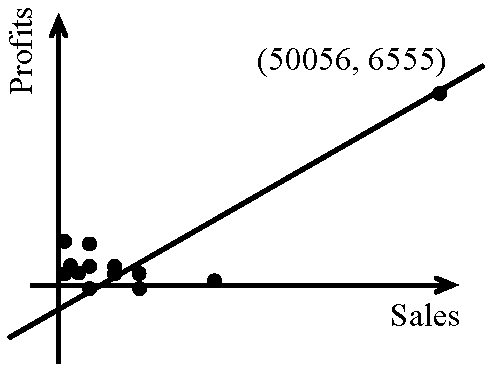 ___y = ax + b
___a = 0.1238, b = 345.8827 ___r² = 0.8732, r = +0.9344 1. Demonstrating your knowledge of the definition of r², explain what the value of r² means in the context of this problem. 2. The teacher who supplied this data set suggested that even though r² is close to one there is reason to doubt some of the interpolative predictive value of this model. He came to this conclusion with no further computation or residual analysis. Explain his reasoning. VI. In assessing the weather prior to leaving our residences on a spring morning, we make an informal test of the hypothesis "The weather will be fair today. "The best" information available to us, we complete the test and dress accordingly. Would be the consequences of a Type I and Type II error? From the choices below select and clearly explain your choice of the correct answer.
|