(Upload on January 30 2026) [ 日本語 | English ]
Mount Usu / Sarobetsu post-mined peatland
From left: Crater basin in 1986 and 2006. Cottongrass / Daylily
HOME > Lecture catalog / Research summary > Glossary > Ordination
|
The apparent complexity of techniques for analyzing vegetation data (Kent & Coker 1992) Plant community data are multivariate in nature = raw data matrix Aims of multivariate analysis
1. Summarizing plant community data 
Reduction of many species/variables into a few components |
[indirect ordination, direct ordination, cluster] Data reductionClassification: Phytosociological approach, Cluster analysis (TWINSPAN)Ordination: direct gradient analysis (CCA), Indirect gradient analysis (PCA,DCA) History1901 Pearson: developed PCA as a regression1927 Spearman: applied factor analysis (to psychology) 1930 Ramensky: introduces the term 'ordnung (German)' into ecology 1954 Goodall DW: introduced PCA into ecology and proposed the term 'ordination' 1970 Whittaker RH (ホイッタカー): developd gradient analysis 1971 Gabriel KR: developd biplot graphical display 1973 Hill MO: re-invented correspondence analysis and introduced CA (as reciprocal averaging) into ecology 1986 ter Braak C: invented CCA |
|
ordinatio (L) ≡ multidimensional scaling, component analysis and latent-structure analysis Ordination (gradient analysis) is one of the popular multivariate analyses an analytical method of ordering samples (plots) and/or species along actual or presumed gradients Normal analysis= R-analysis (R分析): Stand or quadrat ordination Ordination diagram: scatter plot of the eigenvector; used both for biplots and joint plots. Biplot: an ordination diagram of two kinds of entities, e.g., species and environmental variables, which has particular rules of interpretation because it is based on a bilinear model. Interpretation proceeds by projecting points on directions defined by arrows in the biplot. |
Joint plot: an ordination diagram of two kinds of entities based on a weighted averaging method.
Ordination axis: eigenvector, latent variable, theoretical explanatory variable.Inverse analysisor transposed analysis= Q-analysis (Q分析: Species or environmental-factors ordination 
Species score (種スコア): eigenvector coefficient; loading in PCA, center of species curve in CA and DCA. eigenvalue (固有値) = latent roots, characteristic root |
|
To synthesize species or environmental data and to produce an ordination of quadrats based on environmental or species variables alone. Indirect gradient analysis (indirect ordination): internal analysis, "factor analysis", unconstrained ordination, unconstrained multidimensional scaling, possibly followed post-hoc by an regression analysis on external variables Table. Indirect ordination (modified after Kent & Coker 1992)
|
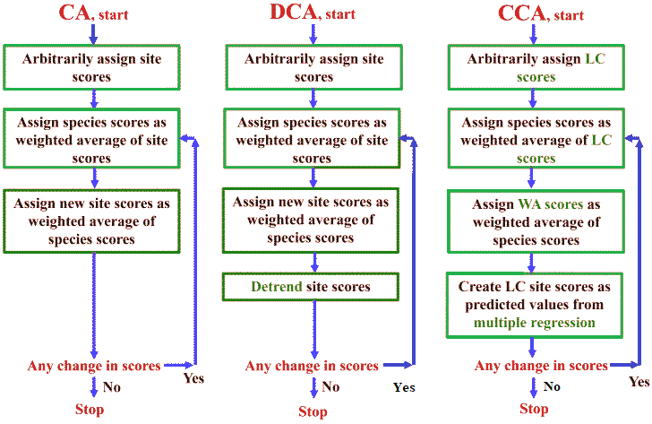 Fig. 1. Algorithms for (A) correspondence analysis, (B) detrended correspondence analysis, and (C) canonical correspondence analysis, diagrammed as flowcharts. LC scores are the linear combination site scores, and WA scores are the weighted averaging site scores. (Palmer 1993) |
Table. Classification of gradient analysis techniques by type of problem, response model and method of estimation. The techniques listed under “linear/least-squares” and “unimodal/weighted averaging” can be carried out with CANOCO.
RESPONSE MODEL: linear unimodal
| Method of estimation: | least-square | maximum likelihood | weighted averaging |
| Type of problem: | |||
| Regression | Multiple regression | Gaussian regression | weighted averaging of site scores (WA) |
| Calibration | linear calibration; "inverse regression" | Gaussian calibration | weighted averaging of species scores (WA) |
| Ordination | Principal component analysis (PCA) | Gaussian ordination | correspondence analysis (CA)5); detrended correspondence analysis (DCA) |
| Constrained ordination1) | Redundancy analysis (RDA)4) | Gaussian canonical ordination | Correspondence analysis (CCA), detrended CCA |
| Partial ordination2) | Partial components analysis | partial Gaussian ordination | partial correspondence analysis; partial DCA |
| Partial constrained ordination3) | Partial redundancy analysis | partial Gaussian canonical ordination | partial canonical correspondence analysis; partial detrended DCA |
Procedure1. make similarity matrix2. Set up two samples that are the lowest similarity on the two poles 3. Calculate scores of the other samples as follows
|
AZ = l = 1.0 - 0.2, KA = d1 = 0.4, KZ = d2 = 0.6 Eigenvaluex:y = kind of contribution rate on axis AZMeasure how much variation in the species data is explained by the particular axis and, hence, by the environmental variables. |
|
PCA: linear response model ↔ CA: unimodal response model Originally defined for data with multi-normal distributions, thus the data should be normalized. Deviations from normality do not necessarily bias the results, however, one should be careful of the descriptors and try to ensure they are not skewed or have outliers. Four versions of PCA
Procedure: Two-way weighted summation algorithm  a. Iteration process 1. Take arbitrary initial site scores (xi), not all equal to zero. 2. Calculate new species scores (bk) by weighted summation of the site scores (Eq 5.8). |
3. Calculate new site scores (xi) by weighted summation of the species scores (Eq 5.9). 4. For the first axis go to step 5. For second and higher axes, make the site scores (xi) uncorrelated with the previous axes by the orthogonalization procedure described below. 5. Standardize the site scores (xi). See below for the standardization procedure. 6. Stop on convergence, i.e., when the new site scores are sufficiently close to the site scores of the previous cycle of the iteration; ELSE go to step 2. 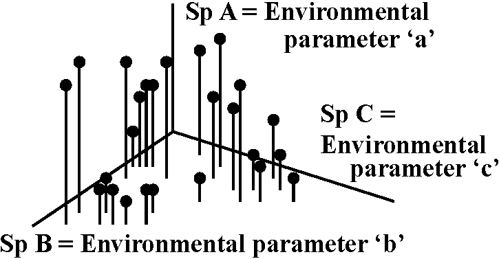 b. Orthogonalization procedure
4.1. Denote the site scores of the previous axis by fi and the trial scores of the present axis by xi. 4.2. Calculate v = Σi=1nxifi. 4.3. Calculate xi, new = xi, old - vfi. 4.4. Repeat Steps 4.1-4.3 for all previous axes. c. Standardization procedure 5.1. Calculate the sum of squares of the site scores s2 = Σi=1nx2. 5.2. Calculate xi, new = xi, old/s Note that, upon convergence, s equals the eigenvalue. |
[ 平均 ]
Weighted averaging method: method based on a unimodal response model (= unimodal trace line) of which the optimum (mode, ideal point) is estimated by weighted averaging. Ex. correspondence analysis.
Procedure
|
Table. Site ordination by weighted average.
                  Site
Species   Weight   1    2    3
  1        100     5    1    0
  2         80     3    3    0
  3         50     2    4    1
  4         30     0    0    3
  5          0    10    0    5
Total             21    9   12
Weighted average  84.0 30.0 15.6
Ex. Site 1: (100 × 5 + 300 × 80 + 50 × 2 + 30 × 0 + 0 × 0)/10Klinka weighted average method
Dry
Wet
Soil moisture indicator index = Weight/Cover × 10 = 15.8 |
|
= reciprocal averaging (反復平均法) 1935 Hartley HO (1912-1980): proposed CA 1973 Benzécri J-P (1932-2019) and colleagues: developed CA |
|
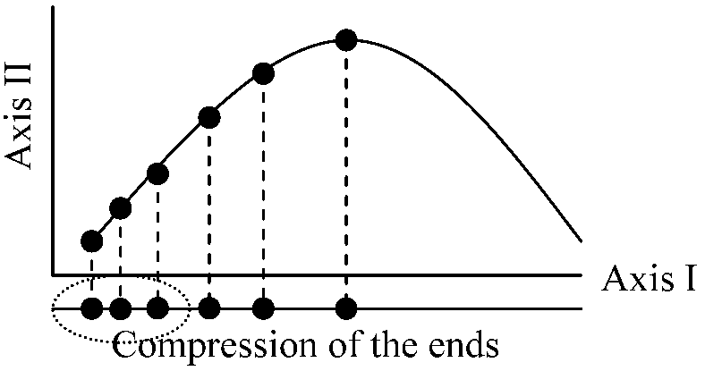
hump = horseshoe (PCA) + arch (CA) + …
Hump can be seen in any PCA and CA The appearance of a projected data swarm as a curve ("arch" or "horseshoe") when the data were obtained from sampling unitHow to remove hump: Do DCA or drop environmental variables highly correlated with the arch to remove the arch. Dropping variables is effective. CANOCO has an improved polynomial detrending technique |
|
Reciprocal averaging, RA= correspondence analysis (Hill 1973)CA is an extension of the method of weighted averaging (Whittaker 1967) → Species commonly show bell-shaped response curves with respect to environmental gradients 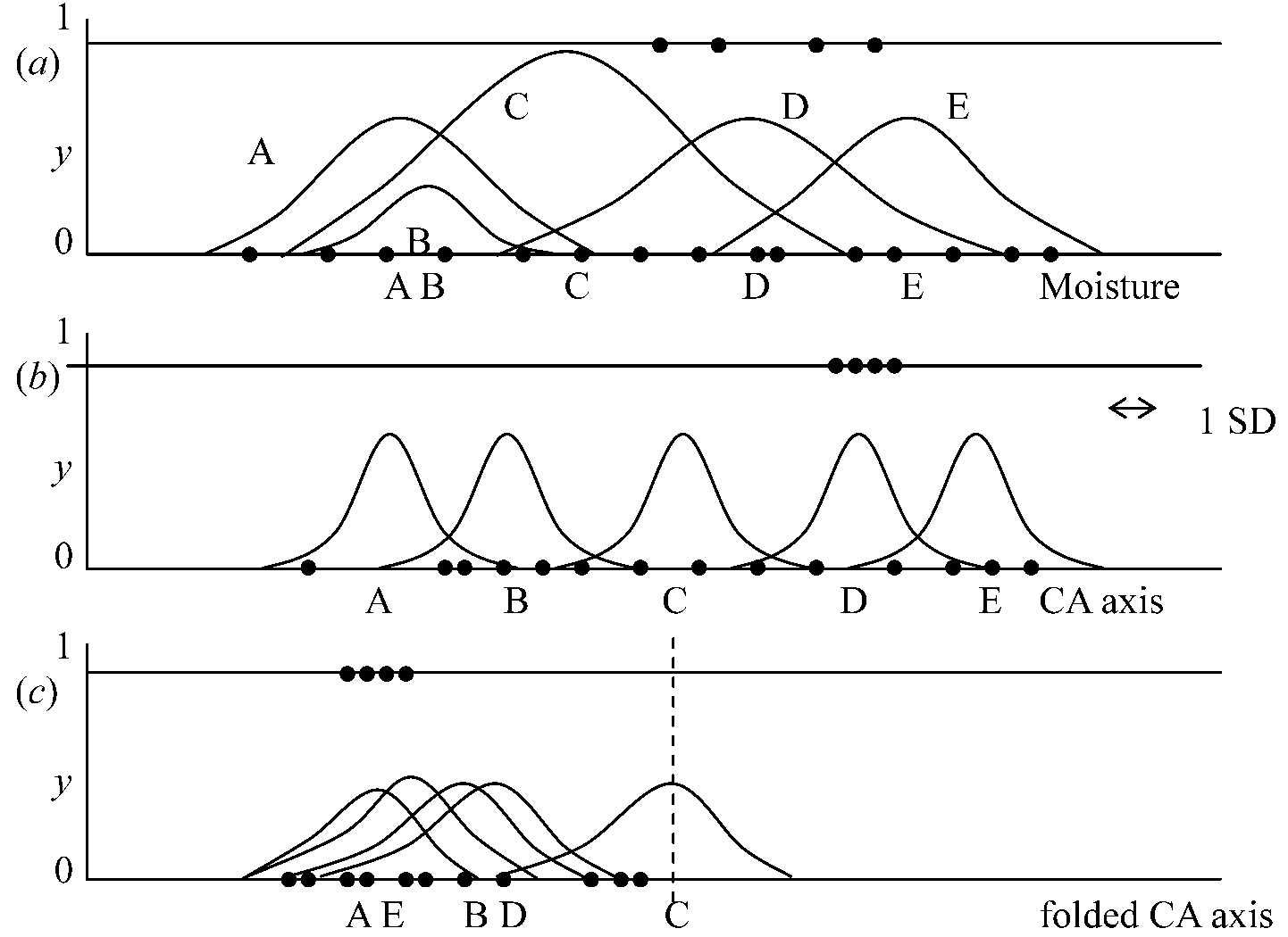 Figure 5.3. Artificial example of unimodal response curves of five species (A-E) with respect to standardized variables, showing different degrees of separation of the species curves, a. real environmental factor, e.g., moisture. b: first axis of CA. c: first axis of CA folded in this middle and the response curves of the species lowered by a factor of about 2. Sites are shown as dots at y = 1 if species D is absent. Procedurea: iteration process (反復過程)1. Take arbitrary, but unequal, initial site scores (xi) 2. Calculate new species scores (uk) by weighted averaging of the site scores (Eq. 5.1). 3. Calculate new site scores (xi) by weighted averaging of the species scores (Eq 5.2). |
4. For the first axis go to step 5. For second and higher axes, make the site scores (xi) uncorrelated with the previous axes by the orthogonaliztion procedure described below. 5. Standardize the site scores (xi). See below for the standardization procedure. 6. Stop on convergence, i.e., when the new site scores are sufficiently close to the site scores of the previous cycle of the iteration; ELSE go to step 2. b: orthogonalization procedure (直交化過程) 4.1. Denote site scores of the previous axis by fi and the trial scores of the present axis by xi. 4.2. Calculate v = Σi=1ny+ixifi/y++, where y+i = Σi=1myki, and y++ = Σi=1ny+i 4.3. Calculate xi, new = xi, old - vfi.4.4. Repeat Steps 4.1-4.3 for all previous axes c: Standardization procedure (標準化過程) 5.1. Calculate the centroid, z, of site scores (xi). z = Σi=1ny+ixi/y++ 5.2. Calculate the dispersion of the site scores s2 = Σi=1ny+i(xi - z)2/y++ 5.3. Calculate xi, new = (xi, old - z)/s Note that, upon convergence, s equals the eigenvalue. Ex. Ecological Statistics Package Detrended correspondence analysis, DCA (Hill 1979)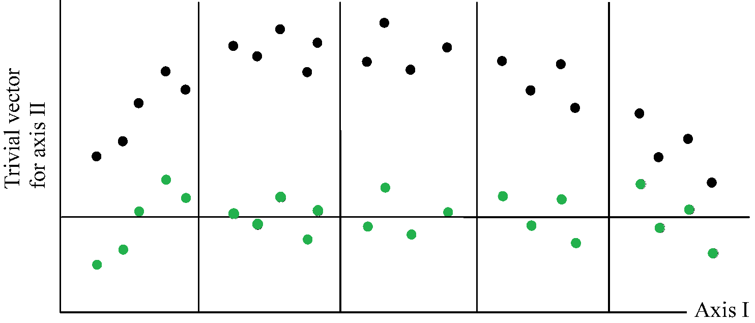 Fig. Method of detrending by segments (simplified). The closed circles indicate site scores before detrending; the open circles are site scores after detrending. The closed circles are obtained by subtracting, within each of five segments, the mean of the trial scores of the second axis (Hill & Gauch 1980). |
Principal coordinate analysis (主座標分析), PCO or PCoA= classical multidimensional scaling (CMDS) |
|
= partial correlation ordination that factors out undesirable influences (like random effects), e.g., difference in observers, phenological variation, block effect, spatial autocorrelation (or depencence) Covariates (covariables): the variables to be factored out |
Partial constrained ordinationspartial CCA, RDA, etcpollution effects × seasonal effects (→ covariables) Eliminate (partial out) effect of covariables. Relate residual variation to pollution variablesReplace environmental variables by their residuals obtained by regressing each pollution variable on the covariables |
| Direct gradient analysis (direct ordination): external analysis, canonical ordination (including DCCA), ordination constrained by external variables, constrained multivariate regression, reduced-rank regression. |
|
Canonical ordination(正準序列化, 適訳無): An ordination in which the axes are constrained to be linear combinations of environmental variables. Designed to detect patterns of variation in the species that can be best explained by the observed environmental variables. Differs from indirect ordination because it incorporates a correlation and regression between floristic data and environmental factors within the ordination analysis. Direct ordination (modified after Kent & Coker 1992) (Detrended) canonical correspondence analysis ([D]CCA)
Not strictly indirect ordination since it is a revised version of DCA with ordination axes constrained by multiple regression with environmental factors. Use CANOCO / CANOPLOT / CANODRAW (Micro$oft Windows version available) for analysis (ter Braak et al. 2002) CCA is widely used technique for direct gradient ordination (ter Braak & Smilauer 2002), assuming that species have a unimodal distribution along environmental gradients. DCCA is the detrended form of CCA, as well as relationship between DCA and CA. |
⇓ CCA (Canonical correspondence analysis) (ter Braak 1987, 1988) Gaussian curve (ガウス曲線, 正常分配曲線): curve expressing erro Distribution - The simplest model for a unimodal species response curve (see explorations in coenospace). It has only three parameters, and the equation is: y = A·exp(-(x-B)2/C), where A is the maximum height of the curve, B is the modal location of the curve, and C is a measure of the breadth of the curve (often called niche breadth, tolerance, or standard deviation). The curve is bell-shaped. The difference between a Gaussian Curve and a Normal Distribution is that the latter is a statistical distribution, and hence the area under the curve is constrained to be one, and the y-axis represents frequency. TerminologyCanonical axis: an ordination axis that is constrained to be a linear combination of environmental variablesCanonical coefficients: parameters of the final regression = the best weights Linear method: method based on a linear model, e.g., linear regression, multiple regression, principal components analysis, redundancy analysis Partial CCAAll the same precautions apply as with CCAOutput will be nearly identical with the inclusion of the variance accounted for by the partial variable.
Total inertial in the ordination - same as CA Packages handling CCA
|
= clustering, classification
A. Hiearchical cluster analysis (階層クラスター分析)1. Aglomerative strategy (bottom-up)Nearest neighbor method (単純連結法, single-linkage method 最近隣法)Mountford average-linkage method (Lassel & Host 1970) Farthest neighbor method (complete-linkage method) Centroid method Median method Ward method (= minimum variance method) 2. Divisive strategy (top-down)Phytosociology - not recommended in generalNomenclature: Weber HE, Moravec J & Theurillat J-P. 2000. International code of phytosociological nomenclature. 3rd edition. Journal of Vegetation Science 11: 739-768 k-meansDIANA (divisive analysis clustering) (Macnaughton-Smith et al. 1964, reviewed by Kaufman & Rousseeuw 1990) Derivations: AGNES, CLARA, DAISY, FANNY, etc. TWINSPAN (two-way indicator species analysis) (Hill 1979)twinspanR in R |
B. Non-hiearchical cluster analysis (非階層クラスター分析) |
|
SITE
TWINSPAN: two-way classification (= both samples and species are grouped), summarizing species distribution across sample groups11 1 219807631245 sp. 9 211-3------- 0000 sp. 5 53415------- 0001 sp. 3 452113------ 0010 sp.11 3254-5------ 0011 sp. 8 -1---53----- 01 sp. 2 -5414545-424 100 sp. 1 231--3221411 101 sp. 6 ----22-23411 1100 sp.10 --142-135553 1101 sp. 7 ----------34 1110 sp.12 ----------54 1110 sp. 4 -----151---- 1111 000000111111 000001001111 00011 010011 00101 0101 01 Table. Output
binary divisive classification
Low - sensitive to subtle differences (over-split), e.g., 0.20
default: 0.00 02.00 5.00 10.00 20.00 |
Eigenvalue: a low eigenvalue indicates that the division is weak
suggesting that the data lacks a clear binary structure or that the cut level is set too high, preventing effective splitting
[ unfold plots along first axis by RA ] ← (1, 3) |
|
= vegetation taxonomy, or syntaxonomy A system for classifying plant communities by means of the tabulation of data collected by quadrats
coverage (被度) Two major schools for phytosociologyScandinavian school (⊃ Uppsala school)emphasized dynamic vegetation processes and successionDu Rietz GE 1885-1967, Sweden: proposed vegetation unit
|
Zurich–Montpellier school (ZM school)developed a rigorous phytosociological classification system based on Braun-Blanquet methodologyFidelity (適合度)= the concentration of a species in a particular syntaxon and which is used both in the classification procedure and in the characterization of syntaxa |