(Upload on May 1 2024) [ 日本語 | English ]
Mount Usu / Sarobetsu post-mined peatland
From left: Crater basin in 1986 and 2006. Cottongrass / Daylily
HOME > Lecture catalog / Research summary > Glossary > Flora
|
Flora (pl. floras or florae) (植物相) The plant species found in one or more regions, or eras (Dunster & Dunster 1996) Fauna (動物相) The animal species found in one or more regions, or eras How to use (Examples)
Flora lists in this siteMount Usu, Mount Koma, Chise-Frep in Shihoro, Plant species in Washington |
Biota (生物相)= fauna + flora
Ex. land biota, benthic biota, African biota |
Based on research in 2000Seventy-five seed plant species (露崎他 2001) Ex. Chimaphila umbellata (L.) W. Barton: collected from the southwestern slope at ca 500 m in elevation at at August 3, 2000. This species generally establish in forests near sea coast. Alpine and/or subalpine plant species Ex. Campanula lasiocarpa Cham.: collected from the southwesten slope at August 3, 2000. This species is an alpine plant. |
Carnivorous plant species Ex. Drosera rotundifolia L.: collected from the southwestern slope at ca 850 m in elevation at August 13, 2000. This species is a typical carnivorous plant. These specimens have been stored in the Hokkaido University Herbarium. What we can say from the flora on Mount Koma
|
[Geography, Island biogeography, GIS]
|
Def. understanding the distribution of species and ecosystems across geographic space and through geological time 1805 Humboldt A: Essai sur la géographie des plantes 1855 DeCandolle A: Géographie botanique raisonée ou exposition de faits principaux et des lois concernant la distribution de plantes de l'époque acuelle 1872 Griesebach: La végétation du globe d'aprés la disposition suivant les climats 1898 Merriam CH: classified North America into six life zones (生物帯), based on elevation and latitude
Arctic-alpine zone: coldest, i.e., tundra and high-altitude vegetation kingdom > region > province > district Def. Ecozone (生物地理区) or biogeographical region
the broadest biogeographic division of the land surface, based on the distribution of organisms - considering evolution Chorotype
AnimalA. Continental distribution typea. Continental chainb. Distribution pattern of taxa over species 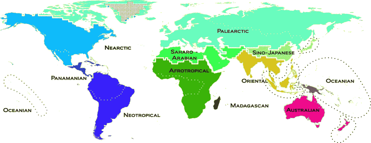 Fig. The terrestrial zoogeographic realms and regions of the world. Zoogeographic realms and regions are the product of analytical clustering of phylogenetic turnover of assemblages of species, including 21,037 species of amphibians, nonpelagic birds, and nonmarine mammals. Dashed lines delineate the 20 zoogeographic regions identified in this study. Thick lines group these regions into 11 broad-scale realms, which are named. Color differences depict the amount of phylogenetic turnover among realms. Dotted regions have no species records, and Antarctica was not included in the analyses (Holt et al. 2013). B. Geographical distribution (地理分布)most popular one is WallaceHuxley (1868): 4 regions
Wallace (1876): 24 subregions in 6 regions, based on the proposal of Sclater, Philip Lutley (1829-1913, ornithologist)
Japan is located on a boundary between Oriental and Palaearctic Region • Holarctic Region (全北区) = Palaearctic + Nearctic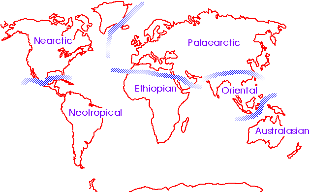 Fig. The original zoogeographical realms. Wallace Line (ウォレス線): the boundary between Oriental and Austrasian Regions
Mammals in in New Guinea - characterized by Australian mammals, e.g., marsupials (wallabies, bandicots and marsupial mice) and monotremes (spiny anteaters) Revised based on Dickerson RE. 1928. Distribution of life in the Philippines. Bureau of printing Weber Line (ウェーバー線) (Weber 1888): rejected the significance of Wallace Line by the distribution of freshwater fish |
Dahl (1925): nine subregions in four regions
Pacific Ocean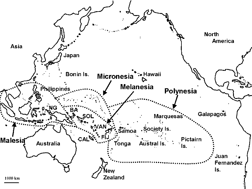 Fig. The Pacific Ocean, showing the biogeographical areas of Malesia, Melanesia, Micronesia and Polynesia (Mueller-Dombois & Fosberg 1998). New Caledonia, Hawaii and New Zealand are not included in Polynesia or Melanesia because of their unique biotas. BA, Bismarck archipelago; CAL, New Caledonia; FIJ, Fiji; NG, New Guinea; SOL, Solomon Islands; VAN, Vanuatu. (Hawaii is included in Polynesia in case.) Melanesia: vlcanoes enclosed by coral reefs in tropical regions Polynesia: coral reefs, except Hawaiian volcanoes Micronesia: coreal reefs with a few voclanoes + Malesia
Insect fauna: characterized by fauna in Oriental Region + islandic factors Floristic Kingdoms (植物区系界)The six floristic kingdoms (Takhtajan 1986)
Japan (日本)Biodiversity hotspots, because of high biodiversityBlakiston Line (ブラキストン線): Tsugaru Strait - mammals and birds named by Milne, John (1850-1913, England) Blakiston, Thomas Wright (1832-1891, England), zoologist (bird)
1857-1859: Palliser Expedition - western Canada animals in Hokkaido are related to northern Asian species Unique plants in Aso (Originally from the Asian Continent)Various unique plants grow in Aso and are rarely seen in other regions. A major characterstic of Aso flora is that among them are a number of plants referred to as living fossils for their origins in North Eastern China and the Korean Peninsula. These plants moved southward from the Asian Continent during the Great Ice Age of 300,000 years ago when Kyushu and Mainland China were joined together and survive today in the cool temperate of the Aso region.Body size on animalsBergmann's rule (ベルクマンの法則)Bergmann, Carl (1814-1865, Germany), anatomist and physiologist1847: body size - temperature
populations and species of larger size are found in colder environments and species of smaller size are found in warmer regions within a broadly distributed taxonomic clade linear and negative relationship between temperature and body weight Allen's rule (アレンの法則)Allen, Joel Asaph (1838-1921, USA), zoologist1877: appendage - climate animals adapted to cold climates have shorter limbs and body appendages than animals adapted to warm climates |
[ University of Hawai'i at Manoa, Botany ]
Characteristics of islandic biotaa) endemic speciesb) disharmonic biota Endemic plantsMetrosideros polymorpha Gaudich. (ハワイフトモモ)well-established on lava |
Exotic plantsmany exotics as well as in Japan and NZEx. Albizia saman (Jacq.) Merr. (monkey pod or rain tree, アメリカネム) Origin: Mexico - Brazil (biologically-invasive species to Hawaii) |
Species distribution models (SDMs)≈ bioclimatic models, climate envelopes, ecological niche models (ENMs), habitat models, resource selection functions (RSFs), range maps, etc.to predici species distribution (Elith & Leathwick 2009) key assumptions = species are at equilibrium with their environments
problems: Basic SDMs
GARP= genetic algorithm for rule-set productionData: using presence/absence data DK-GARPrule sets derived with genetic algorithms, using desktop version PA DesktopGarpBIOCLIMenvelope model (using diva-gis)BRUTOregression, a fast implementation of a GAM (mda in R)DOMAINmultivariate distance, using diva-gis (Carpenter et al., 1993)GBMboosted decision trees, gbm package in RGLMgeneralized linear model, using RMARSmultivariate adaptive regression splines, using mda in R to handle binomial responsesMARSINTmodified MARS, interactions allowed |
MaxEnt model= Maximum entropy model (Phillips et al. 2006)= community assembly by trait selection (CATS) → species distribution and environmental niche modeling
Data
Entropy maximizationtwo parts: a constraint component and an entropy component1) Constraint component
|